Southern California heat advisory extended as triple-digit temperatures persist in inland areas – Pasadena Star News

A heat advisory for much of Southern California was extended through Tuesday evening, June 28, as a heat wave featuring triple-digit temperatures again dominated many inland valleys Monday.

The advisory, which was previously slated to expire at 8 p.m. on Monday, June 27, was extended an additional 24 hours to caution residents that temperatures well above seasonal averages were expected to persist, the National Weather Service said Monday.

⚠️ Heat Advisory extended through Tuesday evening ⚠️ the heat will hang on through the day on Tuesday across inland areas. Please, use caution and check the back seat of your vehicle when leaving. No child or pet should be left in the car for any amount of time.#CAwx pic.twitter.com/NQbaDz3qDg

— NWS San Diego (@NWSSanDiego) June 27, 2022

In Los Angeles County, valley regions experienced consistent high temperatures between the 90 and 100 degree range, said Rich Thompson, meteorologist with the NWS. Some localities broke the 100-degree mark, including a high of 103 in Van Nuys, Thompson said.

Monday’s heat in the San Fernando Valley was on par with weather there on Sunday during the heat wave. Sunday’s highs included 106 in Woodland Hills and 103 in Van Nuys.

The Inland Empire felt “widespread” highs over the triple-digit barrier, with afternoon readings as high as 108 degrees in Chino and 106 degrees in Riverside and San Bernardino, said Dan Gregoria, meteorologist with the NWS. No daily recorded highs were expected Monday though, he said, due to exceptionally high previous records.

“(Today) doesn’t look like record (high) territory, but it still is hot,” Gregoria said.

Uffda, it is hot out today 🥵 here is a look at our 2:30 PM temperatures. What is everyone doing to stay cool today?#CAwx pic.twitter.com/QNukVj5sJM

— NWS San Diego (@NWSSanDiego) June 27, 2022

Inland Orange County high temperatures ranged from the high 80s to the low 90s, according to Gregoria.

On Tuesday, Inland Empire temperatures are expected to continue hovering around the 100-degree mark, with a slight decrease, Gregoria said. The triple-digit highs are expected to finally recede by Wednesday, June 29, but temperatures in the 90s are still expected inland, he said.

Inland Orange County highs are expected to remain in the 80s Wednesday, Gregoria said.

The decreasing highs are part of a cooling trend that is expected to continue through the Fourth of July holiday weekend, Gregoria said. By Saturday, temperatures are projected to be in the 80s for the Inland Empire and in the 70s for much of Orange County, he said.

Swimmers practice at the William J. Woollett Jr Aquatics Center in Irvine on Monday, June 27, 2022. Orange County and inland areas are under a heat advisory until Tuesday night.(Photo by Leonard Ortiz, Orange County Register/SCNG)

Sophia Gonzales, 2, runs through the splash pad at Heritage Community Park in Irvine, CA, on Monday, June 27, 2022. (Photo by Jeff Gritchen, Orange County Register/SCNG)

While high heat warnings when out over much of Southern California, new surfers honed their skills under cool, foggy conditions at the beach near the Santa Monica Pier Monday, June 27, 2022. High temperatures should begin to subside towards the end of the week. (Photo by David Crane, Los Angeles Daily News/SCNG)

Jackson Staley, 2, grabs a rubber duck toy with instructor Joel Velazquez during swimming lesson on a hot day at Shamel Park on Monday June 27, 2022. (Photo by Milka Soko, Contributing Photographer)

A man hydrates at Cabrillo Beach in San Pedro on Monday, June 27, 2022.
(Photo by Axel Koester, Contributing Photographer)

Naja Rajcic learns to windsurf, taking advantage of windy conditions at Cabrillo Beach in San Pedro on Monday, June 27, 2022.
(Photo by Axel Koester, Contributing Photographer)

Jackson Staley, 2, with instructor Joel Velazquez during a swimming lesson on a hot day at Shamel Park on Monday June 27, 2022. (Photo by Milka Soko, Contributing Photographer)

Michael Elias, 5, gets ready to jump at the pool followed by Magnolia Barkley, 4, during a swimming lesson on a hot day at Shamel Park on Monday June 27, 2022. (Photo by Milka Soko, Contributing Photographer)

Kathy Jiménez, 5, kicks during a swimming lesson on a hot day at Shamel Park on Monday June 27, 2022. (Photo by Milka Soko, Contributing Photographer)

A hover glider takes advantage of windy conditions at Cabrillo Beach in San Pedro on Monday, June 27, 2022.
(Photo by Axel Koester, Contributing Photographer)

Children play in La Pintoresca Park’s newly renovated splash pad in Pasadena on Monday, June 27, 2022 during a heat wave. (Photo by Sarah Reingewirtz, Los Angeles Daily News/SCNG)

Ashanty Tebalan, 6, plays in La Pintoresca Park’s newly renovated splash pad in Pasadena on Monday, June 27, 2022 during a heat wave. (Photo by Sarah Reingewirtz, Los Angeles Daily News/SCNG)

With temperatures soaring past 100 degrees, every piece of shade is precious at the North Hollywood metro station Monday, June 27, 2022. High temperatures should begin to subside towards the end of the week. (Photo by David Crane, Los Angeles Daily News/SCNG)

Ximena Pacheco, 10, plays in La Pintoresca Park’s newly renovated splash pad in Pasadena on Monday, June 27, 2022 during a heat wave. (Photo by Sarah Reingewirtz, Los Angeles Daily News/SCNG)

Children play in La Pintoresca Park’s newly renovated splash pad in Pasadena on Monday, June 27, 2022 during a heat wave. (Photo by Sarah Reingewirtz, Los Angeles Daily News/SCNG)

On Monday, some monsoonal moisture entered the region, producing clouds over the mountains in San Bernardino and Riverside counties with the potential for some thunderstorms, Gregoria said. As of 4 p.m., some of the only precipitation seen had been around the Idyllwild area, Gregoria said.

“If anything (thunderstorm related) would develop, the storms would have the tendency to move into the Inland Empire, like around Hemet,” Gregoria said.

Lightning strikes remained a concern throughout mountain areas for possibly sparking brush fires, but no lightning activity had been reported as of early Monday evening, according to the Angeles and San Bernardino national forests.

At least 15 fires were sparked by lightning strikes in the Angeles National Forest by last Wednesday’s storms, said Dana Dierkes, spokeswoman for the Angles National Forest.

One strike smoldered until Friday, June 24, when it emerged as the 3.5 acre Baldy fire, about two miles west of Mt. Baldy in the remote Sheep Mountain Wilderness, the Angeles National Forest reported. As of Monday, the fire had been 80 percent contained, Dierkes said.

Lisa Cox, spokeswoman for the U.S. Forest Service, warned of “sleeper” fires that can linger after lightning strikes.

“These high temperatures and winds kind of wakes them up,” Cox said.

The threat for thunderstorms was expected to linger with the heat wave as well, with an increased chance for precipitation on Tuesday afternoon, Gregoria said.

Tuesday’s forecasted highs:

Man finds iPhone he dropped into river 10 months ago in working condition – BusinessToday

Imagine losing a phone 10 months ago in a river and finding it in working condition. Sounds unbelievable, right? Well, it is not a figment of our imagination but is a true incident. A UK-based man had dropped his iPhone ten months ago in a river. With no hopes of finding it back, he moved on but one day he was informed that his lost phone had been recovered.

As per a BBC report, UK-based Owain Davies had dropped his iPhone into the River Wye near Cinderford, Gloucestershire (UK) in August 2021 during a bachelor party. He probably returned home with the thought of never finding the phone back. Then, almost ten months later, he was contacted by Miguel Pacheco, who went canoeing with his family on the same river. While canoeing, he came across Davies’ iPhone and picked up the lost device from the river. To find the owner of the phone, he posted about the same on Facebook after drying the phone. “I didn’t think it was any good. It was full of water,” he told the BBC.

Despite knowing the phone would probably not restart, he made any attempts to dry the phone because he thought there may have been “sentimental” things on it. “I know if I lost my phone, I’ve got a lot of pictures of my children, I know I’d want that back, ” he said.

However, when he put the device in charge, he couldn’t believe what his eyes saw. The phone started drawing power from the charger and when he switched it on, he saw a screensaver of a man and woman with the date 13 August; the day the phone had fallen into the river. Pacheco’s post about the lost iPhone was shared 4000 times on Facebook, but Davies was not on social media. His friends, however, recognised the phone and helped Davies with connecting with Pacheco.
“I was in a two-man canoe and my partner probably shouldn’t have stood up, and, needless to say, we fell in.The phone was in my back pocket and as soon as it was in the water I realised the phone was gone, Davies told BBC. He also said that he was impressed by all the efforts Pacheco took for his phone.

The iPhones that were launched in recent years are all IP68 rated, which means that the phones can survive up to 1.5 meters of fresh water for 30 minutes, but this was a miracle that does not happen too frequently.

Diagnosis of animal trypanosomoses: proper use of current tools and future prospects | Parasites & Vectors | Full Text

There are critical periods in the course of an infection that are directly associated with the reliability of a diagnosis. For instance, at the onset of an infection, during the first 2–3 weeks after a Trypanosoma infection, any samples analysed by parasite or antibody detection methods may provide false-negative results. Likewise, parasite detection tests in asymptomatic carriers may not reveal the infection, while antibody detection tests would in this case be effective. Conversely, after curative treatment, it may not be possible to ascertain the presence or absence of infection due to the persistence of antibodies in the serum for months [7]. Serial samplings may address such situations.

One or more diagnostic tools need to be used during single or serial sampling to enable a conclusion to be drawn or inference made on a mammal’s status regarding trypanosome infection, whether “non-infected” or “actively infected”, which can either be an “asymptomatic carrier” or a “sick carrier”. As was previously discussed [3], the test specificity can vary, the primers must be selected according to subgenus, species, type and subspecies, and the test results will still remain inconclusive for single or mixed infection status. By using one or more diagnostic tools for serial examinations, it will be possible to differentiate current (parasite ± antibodies) from past infections (antibodies only). Possible outcomes of diagnostic tests regarding the infection and immune statuses are given in Fig. 1.

Fig. 1
figure 1

Parasitaemia in trypanosomes per millilitre (tryp/ml; blue curve) and optical density × 1000 in ELISA (orange curve), modelled in an animal infected by a trypanosome (Trypanosoma evansi in this case) on D0 (Day 0), receiving 1 non-curative treatment on D35, and one curative treatment on D52. See Abbreviation List for the full description of each abbreviation

Parasitaemia in trypanosomes per millilitre (tryp/ml; blue curve) and optical density × 1000 in ELISA (orange curve), modelled in an animal infected by a trypanosome (Trypanosoma evansi in this case) on D0 (Day 0), receiving 1 non-curative treatment on D35, and one curative treatment on D52. See Abbreviation List for the full description of each abbreviation

This figure represents test outcomes from infected animals (T. evansi in cattle, for example) receiving non-curative and curative treatments. Based on the results gathered during experimental infections, we modelled the follow-up of an animal infected on day 0 (D0). In this model, the positive thresholds for the diagnostic techniques were set up as follows: Giemsa-stained thin blood smear (GSBS): 10,000 trypanosomes per millilitre (tryp/ml); haematocrit centrifugation technique (HCT): 100 tryp/ml; PCR-internal transcribed spacer 1 (ITS1): 30 tryp/ml; satellite-DNA PCR: 3 tryp/mll, and enzyme-linked immunosorbent assay (ELISA) optical density (OD) = 0.2. A non-curative treatment was given on D35; this was followed by an “aparasitaemic” period, but the OD in ELISAs remained high. A relapse of the infection was detected from D40 onwards by satellite-DNA PCR, followed by PCR-ITS1 (D46), HCT (D48) and GSBS (D50). A curative treatment on D52 was followed by an “aparasitaemic” period then a progressive decrease, based on OD, until it became negative from D82 onwards. A negative seroconversion 30 days after curative treatment is short; longer periods are generally observed in the field, particularly in older animals having undergone multiple infections. The inconsistency in detection of early infections by the card agglutination test for trypanosomosis (CATT) can be attributed to the presence of immune complexes [8]. On the other hand, it turns negative before the ELISA due to the short half-life of immunoglobulin M (IgM).

Establishment of a “non-infected” status

Due to fluctuating parasitaemia, it is not always possible to demonstrate the presence of trypanosomes in infected animals. Therefore, negative results from parasitological and/or molecular techniques are insufficient to establish a “non-infected” status. Repeated non-detection of antibodies after 1 month (> estimated incubation period of 2–3 weeks) is a stronger criterion.

Immunoglobulin G (IgG) produced against trypanosomes can be detected in the serum from 2 to 3 weeks after infection. According to the recommendations of the World Organisation for Animal Health (WOAH, formerly known as OIE), this is especially true with ELISA plates coated with a complete native antigen, such as whole-cell lysate-soluble antigens (WCLSA) [9, 10]. IgG detection is thus a reliable method for establishing a “non-infected” status in most cases. However, negative parasitological, molecular and serological results are needed twice at a 1-month interval [10].

Nonetheless, a serological test may give a false-negative result in the case of Trypanozoon infections that display occasional extravascular foci, whereby the parasite is not in contact with the immune system [11]. This was hypothesised in the T. evansi camel outbreak that occurred in France [1]. However, such a situation is probably rare and limited to T. evansi in camels. In most cases, accurate indications are obtained from an ELISA, as demonstrated in several validations among different host species. All of these studies agreed on the high sensitivity and reliability of IgG detection by ELISA using WCLSA of trypanosomes [12,13,14,15,16,17,18,19].

In conclusion, with the exception of surra in camels, an unequivocal “non-infected” status can be established (in cattle, buffaloes, horses, sheep, goats, dogs, etc.) if negative results are obtained in a quarantine context, twice at a 1-month interval [9, 10], using: (i) HCT; (ii) one or more molecular detection tests (PCR) selecting the most suitable primers; and (iii) one or more WCLSA ELISA(s), selecting the most suitable species (ELISA T. vivax, T. congolense, T. brucei/T. evansi and/or T. cruzi in Latin America), according to the geographical area and the epizootiological situation [3]. Furthermore, due to its cross-reactivity with all pathogenic mammalian trypanosomes (T. brucei, T. equiperdum, T. vivax, T. congolense and T. cruzi), the T. evansi ELISA test would be an ideal candidate for such screening [17, 20,21,22].

In animals for which no species-specific anti-IgG conjugate is commercially available, protein A-conjugate may be used. However, results using this conjugate have not been fully validated and standardised due to a lack of reference sera from non-infected and infected animals. Consequently, the status of such animals regarding trypanosomosis cannot be certified.

Detection of an “active infection”

Microscopic examinations of GSBSs and buffy coat [23] are quick and cheap ways of detecting active infections. These methods remain the most usual choice in enzootic areas. However, they lack sensitivity and require a minimal level of equipment and skill, which are not always available in the field. Nevertheless, a positive result indicates a parasitaemia > 50–100 tryp/ml, which reflects the immune system’s inability to control the infection and should lead to a treatment decision.

Other parasitological methods, such as the kit for in vitro isolation (KIVI) [24] or the mouse inoculation technique (MIT) (although raising ethical issues), remain the most efficient techniques for parasite isolation [8]. They can be used to demonstrate the parasite’s presence, but also allow further characterisation and storage of field isolates. When applied to diagnosis, they are more sensitive than HCT and GSBS [25], but are relatively expensive and time-consuming. Still, they are helpful for trypanosome isolation during an outbreak in a previously non-endemic area [26] or for high-value animals (racehorses, zoo animals, etc.). The added value of the MIT is clear for Trypanosoma species such as T. evansi and T. brucei that multiply readily in rodents, but for other Trypanosoma species, such as T. congolense and T. vivax, results are inconsistent and, in general, negative for T. equiperdum [27].

Molecular detection of trypanosomes through PCR was a real breakthrough in the development of trypanosome diagnostic techniques in the 1990s [28,29,30]. PCR improved the sensitivity for detecting active infections and significantly improved specificity, at various taxonomic levels. However, molecular methods have critical limitations: (i) they leave cases with low parasitaemia or non-circulating parasites undetected [31, 32]; (ii) they are limited to fully equipped laboratories with skilled technicians; (iii) positive results are conclusive of active infection (leaving aside the fact that DNA may still be detected 24–48 h after curative treatment [33]), but negative results are not; and (iv) there is a significant delay between the time of sampling in the laboratory and the delivery of results, so animals can be out of reach by the time the veterinarian, vet technician or owner receives the results. Loop-mediated isothermal amplification methods (LAMP) applied to parasite DNA can mitigate such drawbacks. Although they were claimed to be efficient and applicable in the field [34,35,36], this has never really been the case. The new polymerase spiral reaction (PSR) method [37] may be suitable for field diagnosis in real time, but it still requires comprehensive field validation. Finally, the new and promising spliced-leader RNA (SL-RNA) detection method is applied to a short and conserved RNA sequence linked to the 5’ end of each trypanosome pre-messenger RNA (mRNA) [38]. Still, its implementation requires expensive equipment for quantitative PCR (qPCR) and skilled personnel [39].

Although antibody detection indicates contact between the host and parasites, it does not confirm active infection, especially as IgG persists several weeks after treatment or self-cure (2–4 months). IgM is produced early and has a short half-life (1–3 months) [8, 40], and is associated with recent infection or recent parasite circulation. IgM detection has a good positive predictive value for detecting active infections, while IgG tests detect an “established infection”. However, IgM immune complexes are captured by phagocytic cells in the serum of actively infected animals and, consequently, IgM detection can give false-negative results [8]. Overall, implementing IgM and IgG detection in a herd showing signs of active infection (positive HCT or PCR) can help identify infected animals, but these methods not suited to detect active infection on their own.

In summary, at the individual level, an active infection can only be established with parasitological (HCT, GSBS, MIT, etc.) and/or molecular tools (PCR, LAMP, PSR, RNA detection, etc.). However, once the infection is confirmed in one or more animals in a group, seropositivity may be considered sufficient by a primary care veterinarian to decide on eliminating parasites, even in apparently healthy animals. Conversely, a “sickness treatment-decision strategy” requires evidence that clinical signs are linked to active infection (see following sections).

Sick or healthy status and treatment decisions

As discussed earlier [3], in enzootic areas (and in the absence of an elimination programme), before deciding on a treatment, a distinction should be made between the “infected and healthy animal” (asymptomatic carrier) and “infected and sick animal” statuses. A meta-analysis aggregation including averaging the results of 180 studies on cattle trypanosomosis in 19 enzootic African countries [41] showed a low prevalence of 15.1% (95% confidence interval: 13.2–17.1). Nevertheless, on a smaller scale, in enzootic areas of Burkina Faso, Cameroon and Ghana, > 50–70% of the cattle are seropositive [42,43,44]. In such areas, a high percentage of cattle are asymptomatic carriers. Therefore, unless there is an ongoing disease elimination programme, despite being seropositive, these animals do not need treatment. A high seropositivity level makes it difficult (if different from tossing a coin) to draw a causal relationship between the presence of anti-trypanosome antibodies and sickness due to trypanosome(s), even in animals with clinical signs compatible with trypanosomosis and other diseases [45]. There are no markers of “trypanosome sickness”. Although a low haematocrit value can help, the sickness may be caused by other agents, such as ticks, Haemonchus spp., haemoparasites, etc. [46]. HCT is an excellent indicator because its low sensitivity indicates a medium to high parasitaemia, suggestive of “insufficient immune control”. Additionally, it may estimate anaemia (low packed-cell volume), which is undoubtedly sufficient reason for trypanocidal treatment.

As microscopes and centrifuges are rarely available in the field, a rapid antigen detection test would help evidence recent circulation of parasites, even with limited sensitivity. Like the T. evansi CATT, card agglutination tests for other Trypanosoma spp., based on IgM, would be of predictive value for trypanosome sickness and support treatment decisions.

Can species and/or subspecies-specific diagnosis be established?

The ELISA offers a large panel of antigens with sensitivity close to or higher than 95% [15, 47, 48] and a high specificity in relation to other genera, such as Anaplasma, Babesia, etc. However, species specificity remains low and strong cross-reactions occur between the main animal trypanosomoses of African origin (ATAO): T. vivax, T. congolense, T. brucei brucei, T. evansi and T. equiperdum [17, 49]. These cross-reactions are due to common antigens shared by salivarian Trypanosoma, but even occur between taxonomically distant species such as T. evansi and T. cruzi [20], or Leishmania [20, 50, 51]. The species specificity of serological tools and therfore “seropositivity” is thus questionable. Fortunately, Megatrypanum such as T. theileri has been shown not to cross-react in an ELISA for trypanosomes [52, 53]. Consequently, ELISAs carried out with WCLSAs of salivarian trypanosomes are specific to “pathogenic Trypanosoma spp.”, but fail to identify them at the species level.

For ATAO control, in most cases−and especially in tsetse-infested areas−a species-specific diagnosis may not be necessary because the control tools (e.g. fly traps and trypanocides) are mostly identical, regardless of the salivarian Trypanosoma species involved. However, knowledge of the infecting Trypanosoma spp. is useful for adjusting the dose and trypanocide to be used. For example: (i) if T. evansi is identified, melarsomine hydrochloride is preferable; (ii) in a nagana area, identifying the species would allow the dose of diminazene aceturate to be adapted to 7 mg/kg for a Trypanozoon infection versus 3.5 mg/kg for an infection by T. vivax or T. congolense.

At the genus level, the co-infection status of an animal seropositive for Trypanosoma spp. or Leishmania spp. antibodies cannot be established using immunodiagnosis due to cross-reactions. In Latin America, cross-reactions should be suspected in studies involving Trypanosoma spp. (T. evansi, T. vivax, T. cruzi, T. equiperdum) and Leishmania spp. Similarly, caution is required with Leishmania and Trypanosoma serological studies in Asia and Africa. Indeed, in Latin America for example, T. vivax and T. evansi ELISAs may react or cross-react due to infection(s) by T. vivax, T. evansi and/or T. cruzi. This is especially so for horses and pigs when using a T. evansi ELISA [54, 55], but also for cattle [56] and buffaloes for both tests [57]. Additionally, Leishmania infections, which may be prevalent in reservoirs such as dogs, are sources of interference [58]. In such cases, the use of species-specific molecular tests and point-of-care diagnostics (POCD) such as recombinant polymerase amplification with lateral flow dipstick (RPA-LFD), recently developed in Mexico for T. cruzi, would be of great value [59]. Furthermore, the recent discovery of Trypanosoma caninum complicates the diagnosis of Trypanosomatidae infections in dogs [60, 61]. In the USA, where T. cruzi [62] and Leishmania [63] are prevalent in horses, interference in serological diagnosis should be suspected, and this situation may also occur in dogs [64].

In Africa, unlike the agents causing nagana, which are considered to be a unique complex entity (at least for their control), species-specific diagnosis may be needed when human pathogens are circulating in animals. It is essential to investigate animal reservoirs to control and eliminate human pathogens [65]. Molecular techniques are well suited for this purpose since they are sensitive and specific. However, PCR may fail to detect infection when primers target a single-copy gene or when using a sample with low parasitaemia. Nested-PCR or RNA detection methods can increase the sensitivity of these tests. Identifying T. b. gambiense and T. b. rhodesiense using subspecies-specific antigen detection would be another option. However, although precise tests may be developed, they would probably have low sensitivity (due to the inverse relationship between sensitivity and specificity), leading to uncertainty when diagnosing negative test results.

Effective and user-friendly tests able to distinguish between all parasites of the subgenus Trypanozoon at the species or subspecies level [66] either have not yet been developed or lack sensitivity. For example, tests to distinguish T. evansi (type A, type B, etc.) from T. equiperdum (type OVI, BoTat, etc.) are inconclusive because of polyphyly [66,67,68,69] or the low sensitivity of the method, which uses single-gene DNA detection tests. In addition, variations in mitochondrial DNA (mtDNA) content (kinetoplastic DNA composed of maxi- and minicircles) can be used to differentiate some Trypanozoon species [70, 71], but the fact that many T. evansi strains are deficient in kinetoplastic DNA (akinetoplastic) [72] limits the widespread use of these tools. Whichever serological test is used (CATT for T. evansi or any of the Trypanozoon ELISAs), in areas of mixed infections, when a positive result suggests a subgenus Trypanozoon infection, it should only be considered a “pathogenic trypanosome infection”. Trypanozoon identification at the subspecies level is possible with DNA-based methods, but at the expense of sensitivity. As an example, positive results are obtained with satellite DNA detection (TBR/NRP primers), which is highly sensitive for Trypanozoon parasites [28, 30] thanks to the 10,000–20,000 sequence repeats. However, specific primers targeting single genes like SRA (T. b. rhodesiense/T. b. brucei) or TGSGP (T. b. gambiense/T. b. brucei) [73, 74]) may be ineffective because of insufficient DNA in the sample. Therefore, when TBR primers provide positive results, the final result will remain inconclusive if single-gene PCRs are negative. PCR sensitivity for diagnosis can thus be ranked as follows: satellite DNA > moderately repeated genes (e.g. ribosomal DNA, ITS1) > single-gene DNA.

When using PCR, a positive test is considered conclusive and a negative one is not, so when the taxon Trypanozoon is detected in a sample, even if one subtaxon is confirmed (e.g. T. evansi using Rode Trypanozoon antigen-type [RoTat]1.2 primers), it will not be possible to detect another Trypanozoon (namely in this example T. equiperdum, T. b. brucei, T. b. rhodesiense or T. b. gambiense) also present in the sample. Thus, a reliable and specific species/subspecies diagnosis may never be established in mixed enzootic hosts and areas.

In conclusion, we urgently need reliable species-specific methods to detect trypanosome infections because of: (i) cross-reactions in antibody detection methods; and (ii) the poor sensitivity of current highly specific DNA-based methods. Even though the epizootiological context would suggest the most probable conclusion (e.g. a trypanosome infection in a horse in the USA is likely to be caused by T. cruzi, while in Asia it would most probably be due to T. evansi), reasonable assumptions may be made only in enzootic areas. Even so, these conclusions cannot be drawn for travelling animals, which could have been exposed to “out of context” parasites. Let us give some rather extreme but also realistic examples. A dog or a racehorse from Africa, which has spent some days in Mexico and then has tested seropositive to an ELISA for T. brucei upon arrival in France should be considered as a potential carrier of one or more of the following pathogens: T. vivax, T. congolense, T. brucei spp., T. evansi, T. equiperdum (for the horse only), T. cruzi and Leishmania spp. [17, 20]. If the same animal has positive PCR results for Trypanozoon, this result confirms it as a carrier of T. brucei spp. and/or T. evansi and/or T. equiperdum. At the same time, it remains suspect for all the other taxa mentioned above due to the PCR’s limited sensitivity.

Although monospecific infections remain the most frequent (thus explaining why we qualified our examples as “extreme”!), to be precise and exhaustive, we must keep in mind the possibility of combined infections. Thus, the only short conclusion on the lack of specificity and sensitivity in trypanosome diagnosis is that once a pathogenic Trypanosoma (or Leishmania) infection is detected, it can hide co-infection(s) by any other pathogenic Trypanosoma (or Leishmania). Such an animal is then a confirmed case of a Trypanosoma infection, in addition to a suspected case of other infection(s) by members of the Trypanosomatidae family.

Diagnosis of trypanosomes in insect vectors

Detecting trypanosomes in insect vectors is feasible for epidemiological studies and risk assessment, but the meanings and limits of any conclusion need to be further discussed.

Trypanosomes can be detected in the mouthparts, salivary glands, midguts, rectum or crushed whole insects, with different significance in terms of development and transmission (mature or immature stage of the cyclical development).

The microscopic observation of trypanosomes in insects does not allow identification of the species since the morphology of insect stages of trypanosomes is not characteristic; therefore, pathogenic trypanosomes may be confused with non-pathogenic ones such as T. theileri (cyclically transmitted by tabanids), or with insect commensals of the Trypanosomatidae family, such as Crithidia [75].

In mechanical vectors

Detecting trypanosomes in the mouthparts of a mechanical vector suggests only a potential for transmission since they can only survive there briefly (30 min to 2 h) [76, 77]. Consequently, detecting trypanosomes in the mouthparts or the midgut of a mechanical vector indicates that the insect fed on an infected animal, but not that the parasite was transmissible to a host. Such information is not particularly relevant; it is easier and more informative to detect trypanosomes in the blood of individual livestock than in blood that is “randomly collected” by an insect. Detecting trypanosomes in haematophagous insects acting as mechanical vectors is therefore of little practical value on livestock farms [75].

However, the situation is different in conservation areas. Since wild animals are difficult to trap or are subject to regulations forbidding their capture, the blood collected by haematophagous insects can be of great interest. Indeed, the detection of trypanosomes in mechanical vectors feeding on wild fauna will provide information on the presence and circulation of these parasites among wild animals and their potential role as reservoirs. In such cases, identifying the insect’s blood meal could provide other complementary information using ELISA [78] or molecular methods, such as PCR amplification of the cytochrome b mtDNA [79]. In addition, it is possible to obtain more information on the vertebrate host through molecular markers or using more recent multiplexed next-generation sequencing (NGS) methods, such as metabarcoding [80, 81]. The application of such methods would notably help to determine the potential circulation of the parasites between host species. However, detection of this kind is rarely implemented due to the low rate of fed insects entering insect traps. This rate could be increased through the use of ultraviolet (UV) light [82], although cost remains a limiting factor.

In cyclical vectors

The case of cyclical vectors of trypanosomes is quite different. When these insects (tsetse flies or triatomine bugs) are found to be “infected” by trypanosomes, the probability that they transmit the parasite is high because they remain permanently infective; their role in the disease epidemiology can thus be addressed and measured [83].

Parasitological methods were the primary tool in the past. They are based on the location of parasites in the vector (gut, salivary glands, proboscis, salivary secretion, faeces) rather than on parasite morphology, which is inconsistent at the insect stages [84]. Molecular techniques have since proved to be more reliable and valuable than parasitological methods for epidemiological studies [85], but contamination during insect dissection could affect detection. Molecular methods are also expensive, especially when considering the total number of PCR tests required per insect, as the number of insect organs is multiplied by the number of Trypanosoma species investigated [85]: 3 × 3 = 9 for (gut + salivary glands + proboscis) × (T. vivax + T. congolense + T. brucei), for example. One option is to dissect the insect and observe body parts through a microscope first, then proceed with PCR tests only for positive samples. Such methods were used to study T. cruzi circulation in Latin America in the framework of large-scale studies to identify biological, ecological and environmental variables associated with Chagas disease [86]. In Africa, they were used to identify pathogenic trypanosomes in tsetse flies [87].

Xenodiagnosis, previously used only for humans [88], is an exciting avenue to explore; it is a sensitive and specific tool to identify trypanosomes in animal and human hosts. Unfortunately, although used for Leishmania [89] and T. cruzi detection in Latin America [90], it has been limited to experimental infections for African trypanosomes [91].

In conclusion, the benefit gained from trypanosome detection in a mechanical vector is limited to wild animals or the interface between livestock and wildlife. More general information can be obtained from tsetse flies and triatomine bugs. Better information should be obtained when combining molecular identification and blood meal analyses [83, 92]. However, the cost of such studies is high since they require insect capture, identification and dissection, (multi-organ) × (multi-species) PCR diagnosis and multi-host blood meal identification [93].

Southern California heat advisory extended as triple-digit temperatures persist in inland areas – San Gabriel Valley Tribune

A heat advisory for much of Southern California was extended through Tuesday evening, June 28, as a heat wave featuring triple-digit temperatures again dominated many inland valleys Monday.

The advisory, which was previously slated to expire at 8 p.m. on Monday, June 27, was extended an additional 24 hours to caution residents that temperatures well above seasonal averages were expected to persist, the National Weather Service said Monday.

⚠️ Heat Advisory extended through Tuesday evening ⚠️ the heat will hang on through the day on Tuesday across inland areas. Please, use caution and check the back seat of your vehicle when leaving. No child or pet should be left in the car for any amount of time.#CAwx pic.twitter.com/NQbaDz3qDg

— NWS San Diego (@NWSSanDiego) June 27, 2022

In Los Angeles County, valley regions experienced consistent high temperatures between the 90 and 100 degree range, said Rich Thompson, meteorologist with the NWS. Some localities broke the 100-degree mark, including a high of 103 in Van Nuys, Thompson said.

Monday’s heat in the San Fernando Valley was on par with weather there on Sunday during the heat wave. Sunday’s highs included 106 in Woodland Hills and 103 in Van Nuys.

The Inland Empire felt “widespread” highs over the triple-digit barrier, with afternoon readings as high as 108 degrees in Chino and 106 degrees in Riverside and San Bernardino, said Dan Gregoria, meteorologist with the NWS. No daily recorded highs were expected Monday though, he said, due to exceptionally high previous records.

“(Today) doesn’t look like record (high) territory, but it still is hot,” Gregoria said.

Uffda, it is hot out today 🥵 here is a look at our 2:30 PM temperatures. What is everyone doing to stay cool today?#CAwx pic.twitter.com/QNukVj5sJM

— NWS San Diego (@NWSSanDiego) June 27, 2022

Inland Orange County high temperatures ranged from the high 80s to the low 90s, according to Gregoria.

On Tuesday, Inland Empire temperatures are expected to continue hovering around the 100-degree mark, with a slight decrease, Gregoria said. The triple-digit highs are expected to finally recede by Wednesday, June 29, but temperatures in the 90s are still expected inland, he said.

Inland Orange County highs are expected to remain in the 80s Wednesday, Gregoria said.

The decreasing highs are part of a cooling trend that is expected to continue through the Fourth of July holiday weekend, Gregoria said. By Saturday, temperatures are projected to be in the 80s for the Inland Empire and in the 70s for much of Orange County, he said.

Swimmers practice at the William J. Woollett Jr Aquatics Center in Irvine on Monday, June 27, 2022. Orange County and inland areas are under a heat advisory until Tuesday night.(Photo by Leonard Ortiz, Orange County Register/SCNG)

Sophia Gonzales, 2, runs through the splash pad at Heritage Community Park in Irvine, CA, on Monday, June 27, 2022. (Photo by Jeff Gritchen, Orange County Register/SCNG)

While high heat warnings when out over much of Southern California, new surfers honed their skills under cool, foggy conditions at the beach near the Santa Monica Pier Monday, June 27, 2022. High temperatures should begin to subside towards the end of the week. (Photo by David Crane, Los Angeles Daily News/SCNG)

Jackson Staley, 2, grabs a rubber duck toy with instructor Joel Velazquez during swimming lesson on a hot day at Shamel Park on Monday June 27, 2022. (Photo by Milka Soko, Contributing Photographer)

A man hydrates at Cabrillo Beach in San Pedro on Monday, June 27, 2022.
(Photo by Axel Koester, Contributing Photographer)

Naja Rajcic learns to windsurf, taking advantage of windy conditions at Cabrillo Beach in San Pedro on Monday, June 27, 2022.
(Photo by Axel Koester, Contributing Photographer)

Jackson Staley, 2, with instructor Joel Velazquez during a swimming lesson on a hot day at Shamel Park on Monday June 27, 2022. (Photo by Milka Soko, Contributing Photographer)

Michael Elias, 5, gets ready to jump at the pool followed by Magnolia Barkley, 4, during a swimming lesson on a hot day at Shamel Park on Monday June 27, 2022. (Photo by Milka Soko, Contributing Photographer)

Kathy Jiménez, 5, kicks during a swimming lesson on a hot day at Shamel Park on Monday June 27, 2022. (Photo by Milka Soko, Contributing Photographer)

A hover glider takes advantage of windy conditions at Cabrillo Beach in San Pedro on Monday, June 27, 2022.
(Photo by Axel Koester, Contributing Photographer)

Children play in La Pintoresca Park’s newly renovated splash pad in Pasadena on Monday, June 27, 2022 during a heat wave. (Photo by Sarah Reingewirtz, Los Angeles Daily News/SCNG)

Ashanty Tebalan, 6, plays in La Pintoresca Park’s newly renovated splash pad in Pasadena on Monday, June 27, 2022 during a heat wave. (Photo by Sarah Reingewirtz, Los Angeles Daily News/SCNG)

With temperatures soaring past 100 degrees, every piece of shade is precious at the North Hollywood metro station Monday, June 27, 2022. High temperatures should begin to subside towards the end of the week. (Photo by David Crane, Los Angeles Daily News/SCNG)

Ximena Pacheco, 10, plays in La Pintoresca Park’s newly renovated splash pad in Pasadena on Monday, June 27, 2022 during a heat wave. (Photo by Sarah Reingewirtz, Los Angeles Daily News/SCNG)

Children play in La Pintoresca Park’s newly renovated splash pad in Pasadena on Monday, June 27, 2022 during a heat wave. (Photo by Sarah Reingewirtz, Los Angeles Daily News/SCNG)

On Monday, some monsoonal moisture entered the region, producing clouds over the mountains in San Bernardino and Riverside counties with the potential for some thunderstorms, Gregoria said. As of 4 p.m., some of the only precipitation seen had been around the Idyllwild area, Gregoria said.

“If anything (thunderstorm related) would develop, the storms would have the tendency to move into the Inland Empire, like around Hemet,” Gregoria said.

Lightning strikes remained a concern throughout mountain areas for possibly sparking brush fires, but no lightning activity had been reported as of early Monday evening, according to the Angeles and San Bernardino national forests.

At least 15 fires were sparked by lightning strikes in the Angeles National Forest by last Wednesday’s storms, said Dana Dierkes, spokeswoman for the Angles National Forest.

One strike smoldered until Friday, June 24, when it emerged as the 3.5 acre Baldy fire, about two miles west of Mt. Baldy in the remote Sheep Mountain Wilderness, the Angeles National Forest reported. As of Monday, the fire had been 80 percent contained, Dierkes said.

Lisa Cox, spokeswoman for the U.S. Forest Service, warned of “sleeper” fires that can linger after lightning strikes.

“These high temperatures and winds kind of wakes them up,” Cox said.

The threat for thunderstorms was expected to linger with the heat wave as well, with an increased chance for precipitation on Tuesday afternoon, Gregoria said.

Tuesday’s forecasted highs:

Qué es la REGLA DE LOS 21 PIES de Tueller

Se maneja en este contexto la llamada regla de Tueller o de los 21 pies (6.4 metros). Esta era la establecida como distancia mínima para tener posibilidades defensivas eficaces con un arma de fuego, enfundada y lista para hacer un disparo, frente a un ataque con arma blanca”

❤️❤️❤️❤️❤️❤️❤️❤️❤️❤️❤️❤️❤️❤️❤️❤️❤️❤️❤️❤️❤️❤️❤️❤️❤️❤️
❤️❤️SI QUIERES APOYAR ECONÓMICAMENTE AL CANAL UNETE ❤️❤️❤️❤️https://www.youtube.com/channel/UCqL9I3dmxX0gc3rSJ0EBz3g/join ❤️❤️

▬▬▬▬▬▬▬▬▬▬ஜ۩۞۩ஜ▬▬▬▬▬▬▬▬▬▬
INSTAGRAM
https://www.instagram.com/battle__guns/
👆👆👆👆👆👆👆👆👆👆👆👆👆👆
▬▬▬▬▬▬▬▬▬▬ஜ۩۞۩ஜ▬▬▬▬▬▬▬▬▬▬
💳💶💶💳💶💶💳💶💶💳💶💶💳💶💶💳💶💶
SITIOS WEB RECOMENDADOS PARA COMPRAR!!!!

– TIENDA DE CONFIANZA: https://absoluteairsoftshop.com/

– LINTERNAS PROFESIONALES SUPER POTENTES (las usa la policía): https://olightstorees.idevaffiliate.com/115.html
🔥10% DTO código: BATTLEAIRSOFT

– Si quieres los mejores SILENCIADORES TRAZADORES: https://acetech.shop

– Si quieres diferentes GADGETS: https://www.airtechstudios.com

– Si quieres nuestras MASCARAS DYE y SUS LENTES: https://www.paintballemboscada.com/es/
🔥10% DTO código: battleairsoft

– Si quieres EQUIPAMIENTO: https://www.tacticalxmen.com
🔥10% DTO código: BAE10

– Si quieres un BREAKPOINT(soporte arma larga) o fundas de EXTRACCIÓN RÁPIDA: contactanos por instagram.

– Si quieres las DIANAS electrónicas que usamos: https://www.r3dproject.es/productos
🔥10% DTO Código: battle
▬▬▬▬▬▬▬▬▬▬ஜ۩۞۩ஜ▬▬▬▬▬▬▬▬
Epidemic Sound, Música Online patrocina. Flexicar, leche de avena
Airsoft, airsoft battle, airsoft war, airsoft gameplay, airsoft españa, airsoft chile, airsoft mexico, airsoft france battle guns

#policia #airsoft #viral #regla21pies

Tagged:

Learning representations of chromatin contacts using a recurrent neural network identifies genomic drivers of conformation | Nature Communications

Hi-C-LSTM representations capture the information needed to create the Hi-C matrix

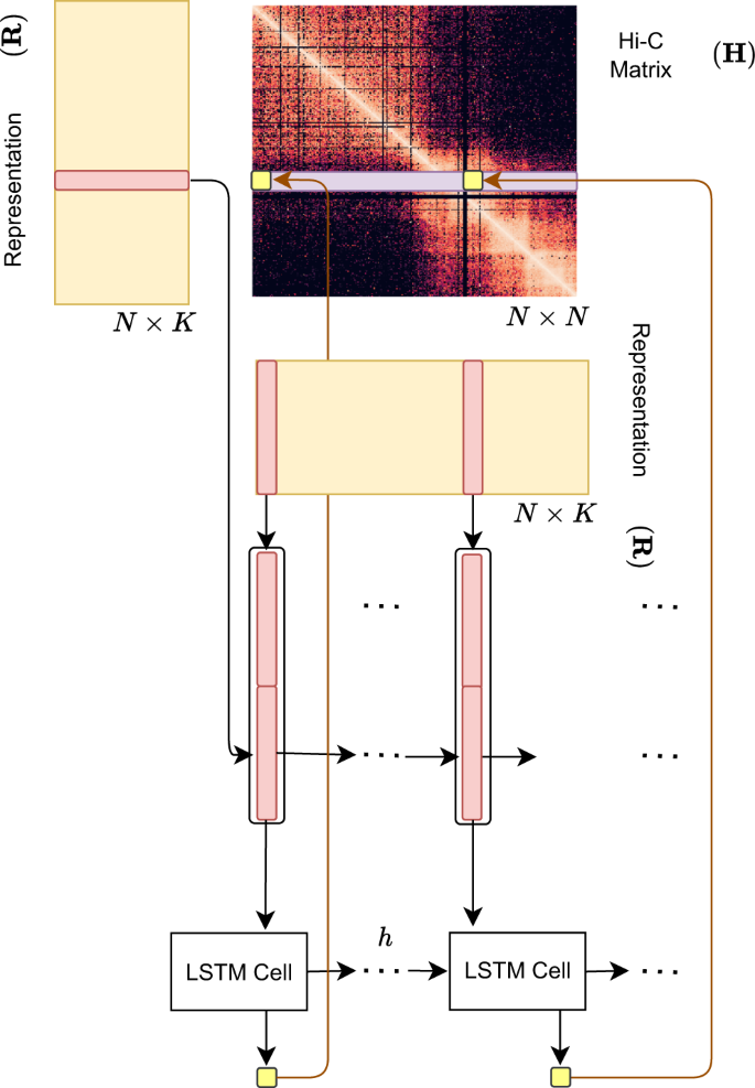
Hi-C-LSTM assigns a representation to each genomic position in the Hi-C contact map, such that a LSTM41 that takes these representations as input can predict the observed contact map (Fig. 2). The representation and the LSTM are jointly trained to optimize the reconstruction of the Hi-C map. This process gives us position-specific representations genome-wide (see the “Methods” section for more details).

Fig. 2: Overview of the Hi-C-LSTM model.
figure 2

A trained Hi-C-LSTM model consists of a K-length representation Ri for each genomic position i and LSTM connection weights (see the “Methods” section). To predict the contact vector of a position i with all other positions, the LSTM iterates across the positions j {1…N}. For each (i, j) pair, the LSTM takes as input the concatenated representation vector (RiRj) and outputs the predicted Hi-C contact probability Hi,j. The LSTM hidden state h is carried over from (i, j) to (i, j + 1). This process is repeated for all N rows of the contact map by reinitializing the LSTM states. The LSTM and the representation matrix are jointly trained to minimize the reconstruction error.

A trained Hi-C-LSTM model consists of a K-length representation Ri for each genomic position i and LSTM connection weights (see the “Methods” section). To predict the contact vector of a position i with all other positions, the LSTM iterates across the positions j {1…N}. For each (i, j) pair, the LSTM takes as input the concatenated representation vector (RiRj) and outputs the predicted Hi-C contact probability Hi,j. The LSTM hidden state h is carried over from (i, j) to (i, j + 1). This process is repeated for all N rows of the contact map by reinitializing the LSTM states. The LSTM and the representation matrix are jointly trained to minimize the reconstruction error.

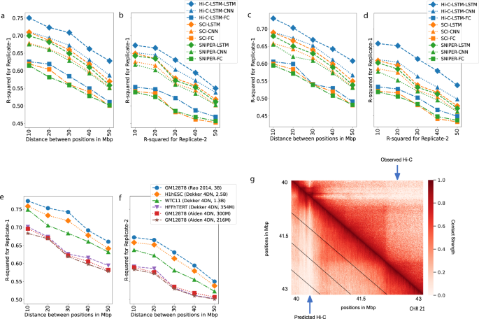
We find that Hi-C-LSTM achieves higher accuracy when constructing the Hi-C matrix compared to existing methods (Fig. 3a, c). The inferred Hi-C map matches the observed Hi-C map (Fig. 3g) closely, and differs from it by about 0.25 R-squared points on average. We adapt SNIPER to our task by replacing the feed-forward decoder that converts low-resolution Hi-C to high-resolution Hi-C with a decoder that reproduces the observed input Hi-C. We call this SNIPER-FC. Hi-C-LSTM outperforms SNIPER (SNIPER-FC) convincingly, by 10% higher R-squared on average (Fig. 3a). Hi-C-LSTM also outperforms SCI (SCI-LSTM) by 12% higher R-squared on average (Fig. 3a).

Fig. 3: Accuracy with which representations reproduce the observed Hi-C matrix.
figure 3

a, b The Hi-C R-squared computed using the combinations of representations from different methods and selected decoders for replicate 1 and 2 (GM12878). The horizontal axis represents the distance between positions in Mbp. The vertical axis shows the reconstruction accuracy for the predicted Hi-C data, measured by average R-squared. The R-squared was computed on a test set of chromosomes using selected decoders with the representations trained all chromosomes as input. The legend shows the different combinations of methods and decoders, read as [representation]-[decoder]. c, d Same as (a, b), but for H1-hESC. e, f Hi-C R-squared computed for different cell types. g A selected portion of the observed Hi-C map (upper-triangle) and the predicted Hi-C map (lower-triangle) in GM12878. The portion is selected from chromosome 21, between 40 and 43 Mbp. Diagonal black lines denote Hi-C-LSTM’s frame boundaries (see the “Methods” section).

a, b The Hi-C R-squared computed using the combinations of representations from different methods and selected decoders for replicate 1 and 2 (GM12878). The horizontal axis represents the distance between positions in Mbp. The vertical axis shows the reconstruction accuracy for the predicted Hi-C data, measured by average R-squared. The R-squared was computed on a test set of chromosomes using selected decoders with the representations trained all chromosomes as input. The legend shows the different combinations of methods and decoders, read as [representation]-[decoder]. c, d Same as (a, b), but for H1-hESC. e, f Hi-C R-squared computed for different cell types. g A selected portion of the observed Hi-C map (upper-triangle) and the predicted Hi-C map (lower-triangle) in GM12878. The portion is selected from chromosome 21, between 40 and 43 Mbp. Diagonal black lines denote Hi-C-LSTM’s frame boundaries (see the “Methods” section).

Two hypotheses could explain Hi-C-LSTM’s improved reconstructions: (1) that Hi-C-LSTM’s representation captures more information, or (2) that an LSTM is a more powerful decoder. We found that both are true. To distinguish these hypotheses, we split each model, respectively, into two components—its representation and decoder—and evaluated each possible pair of components. We train the representations (Hi-C-LSTM, SCI, SNIPER) on all chromosomes and couple them with selected decoders (LSTM, CNN, FC). Using the representations as input, we re-train these decoders with a small subset of the chromosomes and test on the rest. (see the “Methods” section for more details). We compute the average R-squared value for creating the Hi-C contact matrix using each combination of selected representations and decoders

We found that the choice of decoder has the largest influence on reconstruction performance. Using a LSTM decoder performs best, even when using representations derived from SNIPER or SCI (improvement of 0.14 and 0.12 R-squared points on average over fully connected decoders, respectively, Fig. 3a). Furthermore, we found that Hi-C-LSTM’s representations are most informative, even when using decoder architectures derived from SNIPER or SCI (Fig. 3a).

Though the Hi-C-LSTM representations capture important information from a particular sample, we wanted to verify whether they capture real biological processes or irreplicable experimental noise. To check the effectiveness of Hi-C-LSTM representations in creating the Hi-C contact map of a biological replicate, we train the representations on one replicate (replicate 1), repeat the decoder training process on replicate 2 (see the “Methods” section for more details), and compute the average R-squared value for creating the Hi-C contact map of replicate 2 (Fig. 3b, d). The average R-squared reduces slightly for inference of replicate 2 due to experimental variability; however, the performance trend of the representation–decoder combinations is largely preserved (Fig. 3b, d). These results show that Hi-C-LSTM’s improved performance is not merely driven by memorizing irreplicable noise.

We discovered a relationship between sequencing depth and model performance after training and evaluating Hi-C-LSTM on Hi-C datasets from GM12878 with a combined filtered reads of 300 million and 216 million (compared to Hi-C data from Rao et al. which had 3 billion combined filtered reads). We saw that Hi-C-LSTM R2 worsened with reduced read depth, however, the reconstruction performance trend over distance was preserved (Fig. 3e, f).

We also trained and evaluated Hi-C-LSTM on data from 3 other tier 1 cell types from the 4DN Data Portal apart from GM12878, namely, H1-hESC (embryonic stem cell) (Fig. 3c, d), HFF-hTERT (foreskin fibroblast immortalized cell) (Supplementary: Fig. 1a, b), and WTC11 (induced pluripotent stem cell derived from skin leg fibroblast) (Supplementary: Fig. 1c, d). We found that difference in performance across these cell types can be explained by their differing read depths. These data sets have varying read depths, ranging from 150 million (HFFhTERT) to 900 million (H1hESC) filtered reads. We saw that the R2 fell by 0.03 points on average when reads reduced from 3 billion to 1 billion (Fig. 3e). The performance further reduced by 0.4 on average when the reads reduced to 150 million. This amounted to a total R2 decrease of 0.7 points on average with very low sequencing depth (Fig. 3e). We additionally found that the reconstruction performance trend between models is preserved across cell types (Supplementary: Fig. 1).

Hi-C-LSTM representations locate functional activity, genomic elements, and regions that drive 3D conformation

Considering that a good representation of Hi-C should contain information about the regulatory state of genomic loci, we evaluated our model by checking whether these genomic phenomena and regions are predictable from only the representation. Specifically, we test whether the position specific representations learned via the Hi-C contact-generation process are useful for genomic tasks that the model was not trained on, such as classifying genomic phenomena like gene expression42 and replication timing43,44,45,46, locating nuclear elements like enhancers, transcription start sites (TSSs)47 and nuclear regions that are associated with 3D conformation like promoter–enhancer interactions (PEIs)48,49,50, frequently interacting regions (FIREs)51,52, topologically associating domains (TADs), subTADs, and their boundaries18, loop domains and subcompartments18. We compared two classifiers, a boosted decision tree (XGBoost) model53 to predict binary genomic features of GM12878 from representations, for each task separately, and a multi-class multi-label model with a simple linear layer and sigmoid, to predict all tasks from the representations simultaneously (see the “Methods” section for more details regarding comparison methods, baselines and classifiers).

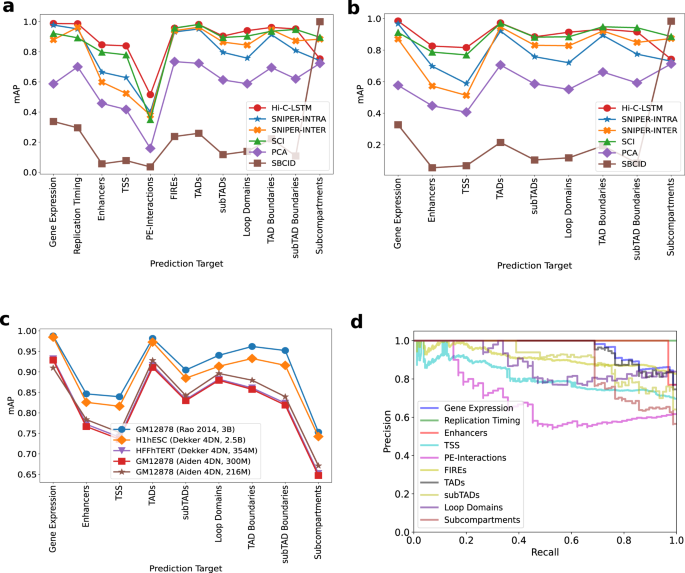
We use mean average precision (mAP) (see the “Methods” section) to quantify classification performance (for additional classification metrics like area under the receiver operating characteristic curve (AuROC), F-score, and Accuracy, refer to the Supplementary, see the “Methods” section for definitions). We find that the models built using the intra-chromosomal representations achieve higher classification performance overall relative to ones trained on inter-chromosomal representations when predicting gene expression, enhancers and TSSs (Fig. 4a, b). This trend is likely due to the relatively close range of the elements involved in prediction. We verify this observation by running Hi-C-LSTM at different resolutions (see the section “Resolution”). In contrast, SNIPER is slightly better at predicting replication timing when compared to the rest of the intra-chromosomal models except Hi-C LSTM (SNIPER-INTER, Fig. 4a, b). While all methods achieve low absolute scores at predicting promoter–enhancer interactions, Hi-C-LSTM performs best (0.5 units on average, 0.1 unit higher on average than SCI) (Fig. 4a, b, d).

Fig. 4: Genomic phenomena and chromatin regions are classified using the Hi-C-LSTM representations as input.
figure 4

a Prediction accuracy for gene expression, replication timing, enhancers, transcription start sites (TSSs), promoter–enhancer interactions (PEIs), frequently interacting regions (FIREs), loop and non-loop domains, and subcompartments in GM12878. The y-axis shows the mean average precision (mAP), the x-ticks refer to the prediction targets, and the legend shows the different methods compared with. b Same as (a), but for targets in H1-hESC. c mAP using Hi-C-LSTM for targets compared across cell types. d The Precision-Recall curves of Hi-C-LSTM for the various prediction targets in GM12878. The y-axis shows the Precision, the x-axis shows the Recall, and the legend shows the prediction targets.

a Prediction accuracy for gene expression, replication timing, enhancers, transcription start sites (TSSs), promoter–enhancer interactions (PEIs), frequently interacting regions (FIREs), loop and non-loop domains, and subcompartments in GM12878. The y-axis shows the mean average precision (mAP), the x-ticks refer to the prediction targets, and the legend shows the different methods compared with. b Same as (a), but for targets in H1-hESC. c mAP using Hi-C-LSTM for targets compared across cell types. d The Precision-Recall curves of Hi-C-LSTM for the various prediction targets in GM12878. The y-axis shows the Precision, the x-axis shows the Recall, and the legend shows the prediction targets.

Both methods perform comparably in predicting the other interacting genomic regions like FIREs, TADs, subTADs, loops domains, and subcompartments (Fig. 4a, b). SNIPER-INTRA as well as SNIPER-INTER do not perform as well as Hi-C-LSTM and SCI on these tasks. One caveat of the model is that it loses CTCF interaction dots at loop boundaries because of its sequential prediction streaks (Supplementary Fig. 2).

The only task on which other methods outperform Hi-C-LSTM is at predicting subcompartments. Subcompartments were originally defined based on inter-chromosomal interactions, so representations based on such interactions outperform those based on intra-chromosomal interactions such as Hi-C-LSTM (see Supplementary: Fig. 3 for confusion matrix). Also subcompartment-ID (SBCID) methods achieves perfect mAP by virtue of its design (Fig. 4a, b). Among the rest of the methods, we find that methods which were designed to predict subcompartments such as SCI and SNIPER-INTER, perform better than the others (Fig. 4a, b). Hi-C-LSTM does perform marginally better than SNIPER-INTRA. Overall, although Hi-C LSTM performs better than other models on most of the tasks, the performance of SCI and SNIPER are comparable to Hi-C-LSTM and all three models perform significantly better than the baselines on average (Fig. 4a, b).

Similar to reconstruction, when comparing classification performance across cell types, we saw that Hi-C-LSTM accuracy worsened with reduced read depth. However, the classification performance trend over tasks was preserved (Fig. 4c). We include results for all available data sets for each cell type. We omitted WTC11 from this analysis because most data sets are not available (see the “Methods” section for details regarding element specific data in cell types). We observed that the accuracy reduced by 0.6 units on average when the reads reduced to 150 million (Fig. 4c). Next, we compared the classification performance of Hi-C-LSTM with other methods (SCI, SNIPER) and baselines (PCA, SUBCOMPARTMENT-ID) in these cell types (Supplementary Figs. 4–6). Similar to R2, we saw that the prediction score trend of methods is preserved across all these cell types.

Understanding what kind of interactions the model is more likely to capture is vital. TADs are identified with a higher accuracy in all cell types compared to other larger chromatin structures like subcompartments (Fig. 4a, b; Supplementary: Fig. 4–6). On the other hand, Promoter-Enhancer interactions are hard to classify in all cell types (Supplementary: Fig. 4,5,6). This means that Hi-C-LSTM representations achieve higher accuracy for medium-scale structures such as TADs than for small-scale structures like promoter–enhancer interactions. This could be due to many factors including data resolution, model architecture, and conservation across cell types.

Hi-C-LSTM recapitulates structures at different Hi-C resolutions

To check if Hi-C-LSTM works at different resolutions of Hi-C data, in addition to our model trained at 10 kbp, we trained Hi-C-LSTM at three other resolutions of 2, 100, and 500 kbp. As expected, models at different scales detect different elements, classify differently, and attribute importance to different sites depending on the resolution. The models achieved these by forming representations that allowed them to construct the Hi-C map at the given resolution. We investigate how these representations differ from the ones learned at 10 kbp.

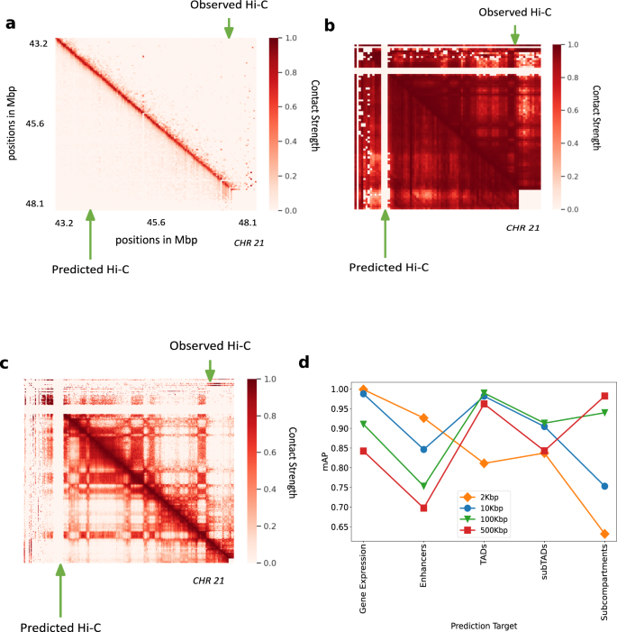
To train the model at 2 kbp, we used only a subset of chromosomes due to memory and compute constraints but trained on the whole genome at other resolutions. A selected portion in chromosome 21 (Fig. 5a) shows that the predicted Hi-C values capture the fine structure of Hi-C even at 2 kbp resolution. The sparsity of available data at 2 kbp is a major constraint in enhancing the performance of the model at this resolution. Hi-C-LSTM captures the Hi-C macro-structures accurately at 500 kbp (Fig. 5b) and 100 kbp (Fig. 5c). This is because operating at this resolution with our sequence length allows it to span entire smaller chromosomes.

Fig. 5: Hi-C-LSTM applied at different resolutions.
figure 5

a Hi-C-LSTM predictions at 2 kbp resolution. A selected portion of the observed Hi-C map (upper-triangle) and the predicted Hi-C map (lower-triangle) in GM12878. The portion is selected from chromosome 21, between 43.2 and 48.1 Mbp. b Hi-C-LSTM predictions at 500Kbp resolution. The observed Hi-C map (upper-triangle) and the predicted Hi-C map (lower-triangle) in GM12878 for chromosome 21. c Hi-C-LSTM predictions at 100 kbp resolution. The observed Hi-C map (upper-triangle) and the predicted Hi-C map (lower-triangle) in GM12878 for chromosome 21. d The classification performance (as measured in mAP) with gene expression, enhancers, TADs, subTADs, and subcompartments of models trained at different resolutions.

a Hi-C-LSTM predictions at 2 kbp resolution. A selected portion of the observed Hi-C map (upper-triangle) and the predicted Hi-C map (lower-triangle) in GM12878. The portion is selected from chromosome 21, between 43.2 and 48.1 Mbp. b Hi-C-LSTM predictions at 500Kbp resolution. The observed Hi-C map (upper-triangle) and the predicted Hi-C map (lower-triangle) in GM12878 for chromosome 21. c Hi-C-LSTM predictions at 100 kbp resolution. The observed Hi-C map (upper-triangle) and the predicted Hi-C map (lower-triangle) in GM12878 for chromosome 21. d The classification performance (as measured in mAP) with gene expression, enhancers, TADs, subTADs, and subcompartments of models trained at different resolutions.

We found that representations at different resolutions predict chromatin structures of different scales. The classification performance (as measured in mAP) with gene expression, enhancers, TADs, subTADs, and subcompartments of models trained at different resolutions (Fig. 5d), shows that for small scale phenomena and expression like gene expression and enhancers, the cumulative prediction score worsens with coarser resolution as expected. For enhancers, the prediction score drops by 0.22 units when the resolution goes from 2 to 500 kbp (Fig. 5d). Both with TADs and subTADs, the model at 100 kbp has the best prediction score, closely followed by the model at 10 kbp (Fig. 5d). We attribute this performance to the fact that these resolutions, combined with our frame length of 150, are close to the to the averages sizes of both these elements. The model at 500 kbp performs best at identifying subcompartments given that the average size of subcompartments is 300 kbp (Fig. 5d). These results point to the idea that aggregating representations learnt at different Hi-C resolutions will likely increase prediction performance across elements of all sizes. Such aggregation will also potentially help in alleviating computational bottlenecks, as a model at a particular resolution need not take the broader context into account (see the section “Discussion”).

Feature attribution reveals association with genomic elements driving 3D conformation

Given that our representations capture elements driving 3D conformation, we should be able to identify those elements using our representations. To validate the ability of our representations to locate genomic regions that drive chromatin conformation, we identified which genomic positions have the largest impact on Hi-C contacts, using the technique of feature attribution. Feature attribution is a technique that allows us to attribute the prediction of neural networks to their input features. In this case, it identifies which genomic positions influence which Hi-C contacts. We ran feature attribution analysis on the Hi-C-LSTM and aggregated the feature importance scores across all the dimensions of the input representation to get a single score for each genomic position (see the “Methods” section for more details). We expected to see higher feature attribution for the genomic elements, regions, domains, and transcription factors (TFs) that are crucial for chromatin conformation.

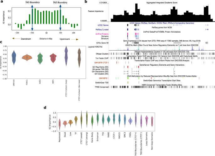
The variation of the aggregated feature importance across interesting genomic regions helps us distinguish boundaries of domains and genomic regulatory elements (Fig. 6a, b). We observe the variation of the feature importance signal across TADs and a selected portion of chromosome 21 (28–29.2 Mbp)54 to check if we can isolate the boundaries of domains, genes and other regulatory elements. To deal with TADs of varying sizes, we partition the interior of all TADs into 10 equi-spaced bins and average the feature importance signal within these bins. We plot this signal along with the signal outside the TAD boundary 50 kbp upstream and downstream, averaged across all TADs (Fig. 6a). The feature importance has largely similar values in the interior of the TAD, noticeably peaks at the TAD boundaries, and slopes downward in the immediate exterior vicinity of the TAD (Fig. 6a). This trend validates the importance of TADs and TAD boundaries in chromatin conformation. We also consider a candidate region in chromosome 21 that is referred to in ref. 54 to observe the variation of feature importance across active genomic elements (Fig. 6b). For this selected region in chromosome 21, as we do not have to deal with domains of varying sizes, we just average the feature importance signal within a specified number of bins and plot this in the UCSC Genome Browser along with genes, regulatory elements, GC percentage, CTCF signal, and conserved TFBS among others. The feature importance peaks around genes, regulatory elements and domain boundaries (Fig. 6b), showing that they play a more important role in conformation than other functional elements. The feature importance peaks also correlate with CTCF peaks and GC percentage peaks (Fig. 6b).

Fig. 6: Hi-C-LSTM representations identify genomic elements involved in conformation through integrated gradients (IG) feature importance analysis.
figure 6

a The IG feature importance averaged across different TADs of varying sizes. The vertical axis indicates the average IG importance at each position and the horizontal axis refers to relative distance between positions in kbp, upstream/downstream of the TADs. b The IG feature importance for a selected genomic locus (chr21 28–29.2 Mbp) along with genes, regulatory elements, GC percentage, CTCF signal, and conserved TFBS among others in the UCSC genome browser. We see that the feature importance scores peak at known regulatory elements, higher GC percentage, and CTCF peaks. c Violin plots of aggregated feature attribution scores for top ranked transcription factor binding sites (TFBS). The x-axis shows the labels/elements and the y-axis displays the z normalized feature importance scores from Integrated Gradients. Both at loop and non-loop regions, the scores shown are aggregated only at shared sites. d Violin plots of aggregated feature attribution scores for selected elements. The x-axis shows the labels/elements and the y-axis displays the z normalized feature importance scores from Integrated Gradients. The scores for CTCF and Cohesin subunits are aggregated genome wide. In c, d, Violin plots present summary statistics where the white dot is the median, thick gray bar is the inter-quartile range, and thin gray line is the rest of the distribution. Kernel density estimation is shown on either side of the line. Sample size for the genomic elements are calculated genome wide by considering all observations of elements according to element specific data.

a The IG feature importance averaged across different TADs of varying sizes. The vertical axis indicates the average IG importance at each position and the horizontal axis refers to relative distance between positions in kbp, upstream/downstream of the TADs. b The IG feature importance for a selected genomic locus (chr21 28–29.2 Mbp) along with genes, regulatory elements, GC percentage, CTCF signal, and conserved TFBS among others in the UCSC genome browser. We see that the feature importance scores peak at known regulatory elements, higher GC percentage, and CTCF peaks. c Violin plots of aggregated feature attribution scores for top ranked transcription factor binding sites (TFBS). The x-axis shows the labels/elements and the y-axis displays the z normalized feature importance scores from Integrated Gradients. Both at loop and non-loop regions, the scores shown are aggregated only at shared sites. d Violin plots of aggregated feature attribution scores for selected elements. The x-axis shows the labels/elements and the y-axis displays the z normalized feature importance scores from Integrated Gradients. The scores for CTCF and Cohesin subunits are aggregated genome wide. In c, d, Violin plots present summary statistics where the white dot is the median, thick gray bar is the inter-quartile range, and thin gray line is the rest of the distribution. Kernel density estimation is shown on either side of the line. Sample size for the genomic elements are calculated genome wide by considering all observations of elements according to element specific data.

We analyzed importance scores at TF binding sites (TFBS)55 and saw that some TFBS have a larger positive importance score compared to others (Fig. 6c). Our motif enrichment analysis showed that the top 5 TFs according to importance score were: CTCF, ZNF143, FOXG1, SOX2, and XBP1 (Fig. 6c). As Cohesin is a known partner of CTCF, we looked for Cohesin-binding sites in the ranked list and found them in the top 15. The full ranked list of transcription factors is attached as a Supplementary file. All TFs in the top 5 are known to play a role in chromatin conformation. The genome folds to form “loop domains”, which are found to be a result of tethering between two loci bound by CTCF and Cohesin subunits RAD21 and SMC340. Among the many models of genome folding, Cohesin ring-associated complex that extrudes chromatin fibers and is delimited by CTCF is most promising. This extrusion model explains why loops do not overlap39.

We found that CTCF + Cohesin sites at loop anchors show 10% higher mean importance score than CTCF + Cohesin sites at non-loop regions (we only considered the case where CTCF and Cohesin share sites) and in both cases they have a spread that is predominantly positive (Fig. 6c). Note that CTCF and Cohesin sites usually overlap, so we analyze them together. Specifically, 98% of loop anchor CTCF ChIP-seq peaks also harbor Cohesin peaks; 92% non-loop CTCF peaks do so56,57. The high feature importance scores observed at CTCF and Cohesin-binding sites reaffirms the crucial role they play in loop formation39,40. The importance of CTCF is further validated by the aggregated feature importance (Fig. 6d), showing a markedly positive score near CTCF-binding sites given by Segway58, particularly the strong ones (mean importance score of 0.45).

Apart from CTCF, the other TFs in the top 5 are also known to play a role in conformation (Fig. 6c). There is a widespread role of C2H2-ZF proteins in chromatin structure and organization59. These TFs are known to promote local chromatin loosening, local chromatin condensation60, and control chromatin accessibility through the recruitment of chromatin-modifying enzymes59. ZNF143 (2nd-most important) is a C2H2-ZF protein. It is known to bind directly to promoters, connect promoters to distal regulatory enhancers61, and plays a partner role in establishing conserved chromatin loops61. Similarly, many FOXG1 (3rd-most important) and related TFs are considered pioneer factors which open closed chromatin and facilitate the binding of other TFs62,63. The last two TFs in our top 5, SOX2 and XBP1, are also known to play a role in conformation. SOX2 loss is seen to decrease chromatin interactivity genome-wide64, and the genomic distribution of XBP1 peaks shows that it binds promoters and potential enhancers65,66.

Along with the aforementioned TFs, we saw that the model places high importance on regulatory elements, particularly enhancers (mean importance score of 0.4) (Fig. 6d). The active domain types had a higher mean score and a spread that largely occupies the positive portion of the feature importance plot when compared to the inactive regions (Fig. 6d). This is further verified by segway-gbr67 feature importance scores (Supplementary Fig. 7). This suggests that active regions may play a dominant role in nuclear organization, where the movement of repressed regions to the periphery is a side-effect.

Aggregated feature importance also demonstrates the largely positive feature attribution of genomic regions that are an integral part of 3D conformation like FIREs, topologically associating domain (TAD) boundaries with and without CTCF sites, loop and non-loop domains (Fig. 6d). TAD boundaries enriched with CTCF show a 20% higher mean importance score compared to TAD boundaries not associated with CTCF, pointing to the importance of CTCF sites at domain boundaries in conformation (Fig. 6d). Moreover, loop domains show a 20% higher mean importance score compared to non-loop domains, which is expected because of the increased contact strength on average and the presence of CTCF sites (Fig. 6d). P-values from the relevant comparisons for each group can be referred to in the Supplementary: Table 1.

Hi-C-LSTM accurately predicts effects of a 2.1 Mbp duplication at the SOX9 locus

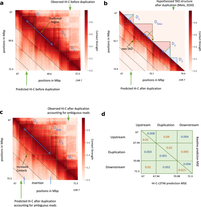
To validate Hi-C-LSTM as a tool for in-silico genome alterations, we simulated a structural variant at the SOX9 locus that was previously assayed by Melo et al. 68. This variant was observed in an individual with Cook’s syndrome and comprises the tandem duplication of a 2.1 Mbp region on chromosome 17 that includes regulatory elements of SOX9 (chr17:67,958,880–70,085,143; GRCh37/hg19, Fig. 7a). To simulate a Hi-C experiment on a genome with this variant, we made a new Hi-C-LSTM representation matrix that includes a tandem copy of the representation at the locus in question and passed this representation matrix through the original Hi-C-LSTM decoder to produce a simulated Hi-C matrix on a post-duplication genome (Fig. 7b). Because Hi-C reads cannot be disambiguated between the two duplicated loci, we simulated mapping reads to the observed hg19 reference by summing reads originating from the two copies (see the “Methods” section). We evaluated Hi-C-LSTM’s predictions according to the agreement between this predicted matrix and a Hi-C experiment performed by Melo et al. 68 (Fig. 7c).

Fig. 7: In-silico duplication of a 2.1 Mbp region on Chromosome 17.
figure 7

In all subplots, upper and lower triangles denote observed and predicted Hi-C contact probabilities respectively, and diagonal black lines denote Hi-C-LSTM frame boundaries. a Observed and predicted Hi-C before duplication. D1, D2 and D3 indicate the three pre-duplication topological domains. b Predicted Hi-C after duplication on a simulated reference genome that includes both copies. Lower triangle indicates Hi-C-LSTM predicted contacts. The true Hi-C contact matrix on this reference genome is not observable because the read mapper cannot disambiguate between the two copies. The upper triangle depicts the post-duplication topological domain structure hypothesized by Melo et al, which includes a novel topological domain DNew. c Observed and predicted Hi-C on the observed pre-duplication reference genome. Upper triangle shows observed post-duplication Hi-C data assayed by Melo et al. Lower triangle shows Hi-C-LSTM predictions, mapped to the pre-duplication reference by summing the contacts for the two copies (see the section “Results”). d Average mean-squared error (MSE) in predicting the observed data by (lower triangle) Hi-C-LSTM, and (upper triangle) a simple baseline (see the section “Results”) at the upstream, duplicated, and downstream regions.

In all subplots, upper and lower triangles denote observed and predicted Hi-C contact probabilities respectively, and diagonal black lines denote Hi-C-LSTM frame boundaries. a Observed and predicted Hi-C before duplication. D1, D2 and D3 indicate the three pre-duplication topological domains. b Predicted Hi-C after duplication on a simulated reference genome that includes both copies. Lower triangle indicates Hi-C-LSTM predicted contacts. The true Hi-C contact matrix on this reference genome is not observable because the read mapper cannot disambiguate between the two copies. The upper triangle depicts the post-duplication topological domain structure hypothesized by Melo et al, which includes a novel topological domain DNew. c Observed and predicted Hi-C on the observed pre-duplication reference genome. Upper triangle shows observed post-duplication Hi-C data assayed by Melo et al. Lower triangle shows Hi-C-LSTM predictions, mapped to the pre-duplication reference by summing the contacts for the two copies (see the section “Results”). d Average mean-squared error (MSE) in predicting the observed data by (lower triangle) Hi-C-LSTM, and (upper triangle) a simple baseline (see the section “Results”) at the upstream, duplicated, and downstream regions.

We found that Hi-C-LSTM accurately predicted the effect of the duplication. The domains that existed pre-duplication (D1, D2, D3, Fig. 7a) are correctly captured post-duplication. In addition, a new chromatin domain (DNew) that was introduced by the duplication is correctly predicted by Hi-C-LSTM (Fig. 7b). To quantitatively evaluate our predictions, we compared them to a baseline that predicts the observed pre-duplication Hi-C for the interactions between the upstream, downstream and duplicated regions, and the genomic average for the interactions of the duplicated region with itself (see the “Methods section). We found that Hi-C-LSTM’s predictions significantly outperform this baseline overall (Fig. 7d). Note the baseline is a slightly better predictor of contacts between the upstream and downstream regions.

Hi-C-LSTM’s predictions have the advantage that they describe contacts on the true post-duplication genome, in contrast to the reference genome used to map reads (Fig. 7c). Hi-C-LSTM’s contacts recapitulate the post-duplication topological domain structure hypothesized by Melo et al. These duplication experiments validate the ability of Hi-C-LSTM to perform in-silico insertion and duplication.

Note that Hi-C-LSTM can simulate only cis effects such as structural variants, but not trans effects that arise from loss of diffusible entities such as transcription factors.

Hi-C-LSTM can simulate knockout of transcription factor binding sites and TAD boundaries

As Hi-C-LSTM is able to perform in-silico insertion/duplication (see the section “Duplication”), we wanted to investigate whether knockout or deletion of certain genomic loci would produce reliable changes in the resulting Hi-C contact map. In-silico knockout experiments have gained prominence lately, mainly in intercepting signal flows in signaling pathways69 and drug discovery70,71,72. A Hi-C in-silico manipulation tool is of great value it enables researchers to identify the importance and influence of any genomic locus of interest to 3D chromatin conformation.

It is an open question how to simulate small-scale perturbations. We performed knockout using four different techniques at CTCF plus Cohesin-binding sites (see the section “Discussion”). The difference in inferred Hi-C between the CTCF plus Cohesin knockout and the no knockout using shifted representations (see the section “Methods”) shows the decrease in contact strength (7% lower on average) in the immediate neighborhood of the KO site (Fig. 8a). Other ways to simulate knockout like using the padding, zero and average representations (Supplementary: Fig. 8) exploit different properties of the model. We believe there is no one right way to perform knockout, however, we prefer the method of shifting all downstream representations from the knockout site upward (see the “Methods” section).

Fig. 8: In-silico deletion of transcription factor binding sites (TFBS), orientation replacement of CTCF binding sites and TAD boundaries with and without CTCF.
figure 8

a The average difference in predicted Hi-C contact strength between CTCF + Cohesin knockout (KO) and no knockout in a 2 Mb window. We simulate deletion by shifting the downstream representations upward. b Average difference in contact strength of the inferred Hi-C matrix between knockout and no knockout (y-axis) for varying distance between positions in Mbp (x-axis). The knockout experiments include TFBS knockout and convergent/divergent CTCF replacements (legend). c The genome-wide average difference in predicted Hi-C contact strength between TAD boundaries knockout and no knockout with CTCF (upper-triangle) and without CTCF (lower-triangle).

a The average difference in predicted Hi-C contact strength between CTCF + Cohesin knockout (KO) and no knockout in a 2 Mb window. We simulate deletion by shifting the downstream representations upward. b Average difference in contact strength of the inferred Hi-C matrix between knockout and no knockout (y-axis) for varying distance between positions in Mbp (x-axis). The knockout experiments include TFBS knockout and convergent/divergent CTCF replacements (legend). c The genome-wide average difference in predicted Hi-C contact strength between TAD boundaries knockout and no knockout with CTCF (upper-triangle) and without CTCF (lower-triangle).

Previous work showed that altering even a single base pair near the loop anchors can make many loops and domains vanish, altering chromatin conformation at the megabase scale39. Given the crucial role played by CTCF and Cohesin subunits in conformation at loop anchors (see sections “Classification”, “Attribution”), we hypothesized that knocking out CTCF and Cohesin subunit binding sites will alter the Hi-C contact map in the neighborhood. The average difference in predicted contact strength between no knockout and knockout at the site under consideration as a function of genomic distance is observed (Fig. 8b). After the combined CTCF and Cohesin knockouts, the average contact strength reduces by 7% in a 200 kbp window when compared to the no knockout case (Fig. 8b). CTCF knockout is seen to affect insulation and reflect possible loss of loops at 200 kbp (Fig. 8b). The knockout of CTCF and Cohesin subunit binding sites at non-loop regions56,57 (just like feature attribution, we only considered the case where CTCF and Cohesin share sites, and ignored the cases where CTCF binds alone, and Cohesin binds alone) produces markedly different effects with 2% lower average inferred strength after knockout at 200 kbp, hinting at the relative importance of loop and non-loop binding factors (Fig. 8b).

Along with CTCF, we knocked out the other 4 TF binding sites (TFBS) in the top 5 TFs according to the ranked list, namely, ZNF143, FOXG1, SOX2, and XBP1 (Fig. 8b). We see that the average predicted contacts after genome-wide knockout partially reflects the importance attributed to each TF by integrated gradients. FOXG1 binding site knockout reduces contacts by 7% on average, XBP1 binding site knockout reduces contacts by 4% on average, whereas ZNF143 and SOX2 binding site knockouts reduce contacts between 4% and 5% on average at 200 kbp. Most knockouts cause an increase in contacts at 300Kbp and a gradual increase in contacts after 400 kbp. These results validate that Hi-C-LSTM knockout of TFBS captures the general idea of contacts depleting within the domain and connecting regions outside the domain.

The CTCF sites at loop anchors occur mainly in a convergent orientation, with the forward and reverse motifs together, suggesting that this formation maybe required for loop formation18,73,74,75,76,77,78 (see Supplementary Fig. 9 for illustration). To check how important the orientation of CTCF motifs is to conformation, we conducted CTCF orientation replacement experiments at loop boundaries. The average difference in predicted contact strength between no replacement and replacement at the site under consideration as a function of genomic distance is observed (Fig. 8b). The replacement of convergent with the divergent orientation around loops is seen to behave similar to the case of CTCF knockout thereby validating observations made in79 (Fig. 8b). On the other hand, replacement of divergent with the convergent orientation is seen to preserve loops at 200 Kbp and behave similar to the control (Fig. 8b).

TADs anchored with CTCF at their boundaries have a differential role to play in conformation compared to the TADs without CTCF. We wanted to check if Hi-C-LSTM can capture this differential behavior of TADs by knocking out their boundaries. To deal with TADs of varying sizes, we partition the interior of all TADs into 10 equi-spaced bins and average the predicted contacts within these bins. We show these along with the regions outside the TAD boundary 100Kbp upstream and downstream, averaged across all TADs (Fig. 8c). The average difference in inferred Hi-C between the knockout at TAD boundaries and the no knockout (Fig. 8c) shows largely decreased contacts for both TADs with and without CTCF in a 200 kbp window (3% lower on average). Within the TAD, however, we see increased contacts for TADs without CTCF (5% higher on average) and decreased contacts with CTCF (4% lower on average) (Fig. 8c).

Simulating loop anchor deletions at the TAL1 and LMO2 loci Hi-C-LSTM predicts measured 5C data

To further validate the ability of Hi-C-LSTM to predict experimental perturbations, we simulated the deletion of loop anchor regions at the TAL1 and LMO2 neighborhood boundaries in human embryonic kidney cells (HEK-293T) previously conducted by Hnisz et al.80. These deletions were observed in T-cell acute lymphoblastic leukemia (T-ALL) patients. The TAL1 anchor deletion was seen on chromosome 1 in the neighborhood of 47.7 Mbp (GRCh37/hg19, Fig. 9a), and the LMO2 anchor deletion was seen on chromosome 11 in the neighborhood of 34 Mbp (GRCh37/hg19, Fig. 9b)80. Both deletions included loop boundary sites. The authors hypothesized that deletions of loop boundary sites at these loci could cause activation of inactive proto-oncogenes within the loops80. To simulate a Hi-C experiment on a genome with these deletions, we first obtained the trained model from GM12878 and retrained it on the 5C data from the TAL1 and LMO2 segments80. We then made a new representation matrix that shifted the representations downstream from the knockout sites upward, and passed this representation matrix through the retrained Hi-C-LSTM decoder to produce a simulated Hi-C matrix (Supplementary Fig. 10a, b, lower-triangle) (see the “Methods” section for more details) and compared this with the 5C experiment performed by Hnisz et al. 80 (Supplementary Fig. 10a, b, upper-triangle).

Fig. 9: In-silico anchor deletions at the TAL1 and LMO2 loci.
figure 9

a, c TAL1 anchor deletion on chromosome 1. a Observed Hi-C contacts before deletion (upper-triangle), and predicted Hi-C contacts before deletion (lower-triangle). c Scatter plot of differences in contacts after and before TAL1 deletion. The x-axis shows observed differences, and the y-axis shows predicted differences. b, d LMO2 anchor deletion on chromosome 11. b Observed Hi-C contacts before deletion (upper-triangle), and predicted Hi-C contacts before deletion (lower-triangle). d Scatter plot of differences in contacts after and before LMO2 deletion. The x-axis shows observed differences, and the y-axis shows predicted differences, KO knockout, WT wild-type.

a, c TAL1 anchor deletion on chromosome 1. a Observed Hi-C contacts before deletion (upper-triangle), and predicted Hi-C contacts before deletion (lower-triangle). c Scatter plot of differences in contacts after and before TAL1 deletion. The x-axis shows observed differences, and the y-axis shows predicted differences. b, d LMO2 anchor deletion on chromosome 11. b Observed Hi-C contacts before deletion (upper-triangle), and predicted Hi-C contacts before deletion (lower-triangle). d Scatter plot of differences in contacts after and before LMO2 deletion. The x-axis shows observed differences, and the y-axis shows predicted differences, KO knockout, WT wild-type.

They authors saw that the insulated neighborhoods of TAL1 and LMO2 were disrupted, which allowed activation of these elements by regulatory elements outside the loop, and caused rearrangement of interactions around the neighborhood. We found that Hi-C-LSTM’s predicted contacts correlate with the post-deletion interactions hypothesized by Hnisz et al. To evaluate our predictions, we investigated whether there is a correlation in the differences of knockout and no knockout between the observed and the predicted contacts (Fig. 9c, d). We found a noticeable correlation between Hi-C-LSTM’s prediction differences between knockout and no knockout and the observed assayed contacts for TAL1 (Fig. 9c). The interactions across domain boundaries that did not exist pre-deletion in the TAL1 neighborhoods were correctly captured by Hi-C-LSTM (Fig. 9c). The correlation for LMO2 was not as strong as TAL1 (Fig. 9d) and the discrepancy was particularly at points where the post knockout contacts were same as the pre-knockout or higher. We see that Hi-C-LSTM accurately predicts decrease in post knockout contacts as decrease, but wrongly attributes some points of no-change and increase as decrease (Fig. 9d).

These anchor deletion experiments reaffirm that Hi-C-LSTM can perform in-silico alterations with moderate accuracy. Moreover, the results also point to the transfer learning ability of Hi-C-LSTM in cell types with limited data (see the section “Discussion”).

$${\rm {cf}} =\frac{1}{v+\delta }\\ {\rm {CP}} =\exp (-a* {\rm {cf}}),$$

Frequently interacting region (FIRE) scores were converted to binary indicators using 0.5 as a threshold following95. See the section “Data availability” for links to FIRE data.

An LSTM’s output is determined by the following series of operations41.

$${{{{{{{{\boldsymbol{f}}}}}}}}}_{{{{{{{{\boldsymbol{t}}}}}}}}} =\sigma ({{{{{{{{\boldsymbol{W}}}}}}}}}_{{{{{{{{\mathbf{f}}}}}}}}}{{{{{{{{\boldsymbol{x}}}}}}}}}_{{{{{{{{\boldsymbol{t}}}}}}}}}+{{{{{{{{\boldsymbol{U}}}}}}}}}_{{{{{{{{\mathbf{f}}}}}}}}}{{{{{{{{\boldsymbol{h}}}}}}}}}_{{{{{{{{\boldsymbol{t}}}}}}}}-{{{{{{{\bf{1}}}}}}}}}+{{{{{{{{\boldsymbol{b}}}}}}}}}_{{{{{{{{\mathbf{f}}}}}}}}})\\ {{{{{{{{\boldsymbol{i}}}}}}}}}_{{{{{{{{\boldsymbol{t}}}}}}}}} =\sigma ({{{{{{{{\boldsymbol{W}}}}}}}}}_{{{{{{{{\mathbf{i}}}}}}}}}{{{{{{{{\boldsymbol{x}}}}}}}}}_{{{{{{{{\boldsymbol{t}}}}}}}}}+{{{{{{{\boldsymbol{{U}}}}}}}_{{\mathbf {i}}}}}{{{{{{{{\boldsymbol{h}}}}}}}}}_{{{{{{{{\boldsymbol{t}}}}}}}}-{{{{{{{\bf{1}}}}}}}}}+{{{{{{{{\boldsymbol{b}}}}}}}}}_{{{{{{{{\mathbf{i}}}}}}}}})\\ {{{{{{{{\boldsymbol{o}}}}}}}}}_{{{{{{{{\boldsymbol{t}}}}}}}}} =\sigma ({{{{{{{{\boldsymbol{W}}}}}}}}}_{{{{{{{{\mathbf{o}}}}}}}}}{{{{{{{{\boldsymbol{x}}}}}}}}}_{{{{{{{{\boldsymbol{t}}}}}}}}}+{{{{{{{{\boldsymbol{U}}}}}}}}}_{{{{{{{{\mathbf{o}}}}}}}}}{{{{{{{{\boldsymbol{h}}}}}}}}}_{{{{{{{{\boldsymbol{t}}}}}}}}-{{{{{{{\bf{1}}}}}}}}}+{{{{{{{{\boldsymbol{b}}}}}}}}}_{{{{{{{{\mathbf{o}}}}}}}}})\\ {{{{{{{{\boldsymbol{c}}}}}}}}}_{{{{{{{{\boldsymbol{t}}}}}}}}} ={{{{{{{{\boldsymbol{f}}}}}}}}}_{{{{{{{{\boldsymbol{t}}}}}}}}}\circ {{{{{{{{\boldsymbol{c}}}}}}}}}_{{{{{{{{\boldsymbol{t}}}}}}}}-{{{{{{{\bf{1}}}}}}}}}+{{{{{{{{\boldsymbol{i}}}}}}}}}_{{{{{{{{\boldsymbol{t}}}}}}}}}\circ \sigma ({{{{{{{{\boldsymbol{W}}}}}}}}}_{{{{{{{{\mathbf{c}}}}}}}}}{{{{{{{{\boldsymbol{x}}}}}}}}}_{{{{{{{{\boldsymbol{t}}}}}}}}}+{{{{{{{{\boldsymbol{U}}}}}}}}}_{{{{{{{{\mathbf{c}}}}}}}}}{{{{{{{{\boldsymbol{h}}}}}}}}}_{{{{{{{{\boldsymbol{t}}}}}}}}-{{{{{{{\bf{1}}}}}}}}}+{{{{{{{{\boldsymbol{b}}}}}}}}}_{{{{{{{{\mathbf{c}}}}}}}}})\\ {{{{{{{{\boldsymbol{h}}}}}}}}}_{{{{{{{{\boldsymbol{t}}}}}}}}} ={{{{{{{{\boldsymbol{o}}}}}}}}}_{{{{{{{{\boldsymbol{t}}}}}}}}}\circ \sigma ({{{{{{{{\boldsymbol{c}}}}}}}}}_{{{{{{{{\boldsymbol{t}}}}}}}}})$$

A trained Hi-C-LSTM model consists of LSTM parameters (see section “LSTM”) and a representation matrix \(R\in {{\mathbb{R}}}^{N\times M}\), where M is the representation size. At each genomic position, (i, j) pair is given as input to an embedding layer, which indexes the row and column representations \({{{{{{{{\boldsymbol{R}}}}}}}}}_{{{{{{{{\boldsymbol{i}}}}}}}}},{{{{{{{{\boldsymbol{R}}}}}}}}}_{{{{{{{{\boldsymbol{j}}}}}}}}}\in {{\mathbb{R}}}^{M}\) and feeds these two vectors as input to the LSTM. The output of the LSTM is the predicted Hi-C contact probability \({\hat{H}}_{i,j}\) for the given (i, j) pair.

The hidden states of the LSTM are carried over from preceding columns thereby maintaining a memory for the row. For the sake of memory usage, the hidden states are reinitialized after every each frame of 1.5 Mbp or 150 resolution bins (see section “Modeling Choices”). This process is repeated for each row of the Hi-C matrix (Eq. (3)).

$${{{{{\rm{MS{E}}}}}}}_{i}=\frac{1}{N}\left[\mathop{\sum}\limits_{j=1}^{N}{\left({H}_{i,j}-{\hat{H}}_{i,j}\right)}^{2}\right]\,{{{{{\rm{for}}}}}}\,i=1,2,\ldots ,N$$

We employed PyTorch, a Python-based deep learning framework and trained Hi-C-LSTM on GeForce GTX 1080 Ti GPUs with ADAM as the optimizer105. All parameters in PyTorch were set to their default values while training. As our primary goal was not to infer values for unseen positions but to form reliable representations for every chromosome, we trained our model on the full genome. For our Hi-C reproduction evaluation, we trained the representations on the full genome but the decoders only on a random subset. We chose to train the decoders on a random subset of the genome to prevent the decoder from overpowering the representations. The time taken to train and test all methods is included in the Supplementary Table 3 (Running Time).

To choose the representation size of our model, we performed an ablation analysis. We computed the average mAP across all downstream tasks with the Hi-C-LSTM model which consists of a single layer, unidirectional LSTM with layer norm in the absence of dropout106 for odd chromosomes and used the even chromosomes to validate whether the choice of hyperparameters remained the same irrespective of chromosome set. We observed the mAP (see “Methods” section) of the Hi-C-LSTM vs. increasing representation size along with Hi-C-LSTM that is bidirectional, in the presence of dropout, without layer norm and 2 layers (Supplementary Fig. 13). While both the presence of dropout and the absence of layer norm adversely affected mAP, the addition of a layer and a complimentary direction did not yield significant improvements in downstream performance. We conducted a similar ablation experiment and computed the average Hi-C R-squared for the predictions with increasing representation size (Supplementary Fig. 13) and observed that the performance trend is preserved, which was indicative of the fact that recreating the Hi-C matrix faithfully aids in doing well across downstream tasks. These results were verified to be true for even chromosomes as well (Supplementary Fig. 13). For both odd and even chromosomes, even though the Hi-C prediction accuracy increased with hidden size, we noticed the elbow at a representation size of 16 for average mAP and therefore set our representation size to that value as a trade-off.

We investigated three hypotheses with following analysis. First, we asked whether the Hi-C-LSTM representations faithfully construct the Hi-C matrix. Second, whether the Hi-C-LSTM representation and the decoder are both powerful in generating the Hi-C map. Third, we evaluated the utility of the representations to infer a replicate map. In all cases, we computed the average prediction accuracy in reconstructing the Hi-C contact matrix, measured using R-squared, which represents the proportion of the variance of the observed Hi-C value that’s explained by the Hi-C value predicted by the Hi-C-LSTM. We sampled the means of observed Hi-C values at different distances between positions and used that as a baseline.

In our second experiment (Fig. 3b), we trained the representations on replicate 1 using all chromosomes, and repeated the aforementioned decoder training process on replicate 2.

We conducted both these experiments in all 4 cell types, namely, GM12878 (Fig. 3a, b), H1-hESC (Fig. 3c, d), HFF-hTERT (Supplementary Fig.1a, b), and WTC11 (Supplementary Fig.1c, d).

For each type of element, we first trained a boosted decision tree classifier called XGBoost53 on the representations. We tried tree boosting first as it is shown to outperform other classification models with respect to accuracy when ample data is available. Following Avocado95, we used XGBoost with a maximum depth of 6 and a maximum of 5000 estimators and these parameters were chosen following ablation experiments with odd chromosomes as the training set and even chromosomes as the test set (Supplementary Fig. 15). N-fold cross-validation, with n = 5, was used to validate our training with and an early stopping criterion of 20 epochs. The rest of the XGBoost parameters were set to their default values.

For each task, the genomic loci under contention were assigned labels. All tasks were treated as binary classification tasks, except the subcompartments task, which was treated as a multi-class classification task. For tasks without preassigned negative labels, negative labels were created by randomly sampling genome-wide, excluding the regions with positive labels. We sampled negative labels until the number of negative labels equaled the number of positive labels to avoid class imbalance during classification. The XGBoost classifier was given the representations at these genomic loci as input and the assigned labels as targets.

We then compared the XGBoost classifier trained separately for each task with a multi-class multi-label classifier with a simple linear layer and sigmoid output. We observed that the multi-class classifier, which predicted regions/domains the given position belonged to, was much faster and gave more reliable results when compared to the XGBoost classifier. Therefore, we prefer the linear classifier for classification.

The classifiers were evaluated using four standard metrics for classification tasks, namely, mean average precision (mAP) (otherwise known as area under the Precision-Recall curve (AuPR)), area under the Receiver Operating Characteristic curve (AuROC), Accuracy (\(A=\frac{{\rm {TP+TN}}}{\rm {{TP+FP+TN+FN}}}\)), and F-score. AuROC is defined as the area under the curve that has true positive rate (\({\rm {TPR}}=\frac{{\rm {TP}}}{{\rm {TP+FN}}}\)) on the y-axis and false positive rate (\({\rm {FPR}}=\frac{\rm {{FP}}}{\rm {{FP+TN}}}\)) on the x-axis. mAP is defined as the average of the maximum precision (\(P=\frac{{\rm {TP}}}{\rm {{TP+FP}}}\)) scores achieved at varying recall levels (R = TPR). F-score is defined based on precision and recall (\(F=\frac{2P* R}{P+R}\)). We compared these metrics for GM12878, H1-hESC, and HFF-hTERT (see Supplementary Figs. 4–6 for more details).

$${{{{{\rm{I{G}}}}}}}_{{{{{{\rm{norm}}}}}}}=\frac{{{{{{\rm{IG}}}}}}-{{{{{\rm{IG}}}}}}_{{{{{\rm{min}}}}}}}{{{{{{\rm{IG}}}}}}_{{{{{\rm{max}}}}}}-{{{{{\rm{IG}}}}}}_{{{{{\rm{min}}}}}}}.$$

The Hi-C-LSTM enables us to perform in-silico deletion, orientation replacement and reversal of genomic loci and predict changes in the resulting Hi-C contact map. We performed three types of experiments:: knockout, CTCF orientation replacement, and duplication. In a knockout experiment, we chose certain genomic sites (such as CTCF and Cohesin binding sites) and replaced their representations with a different representation depending on the method used to perform the knockout (Supplementary Fig. 8).

Among the four possible methods to perform knockout, we prefer the method of shifting the representations. Shifting the representations not only captures the true post-duplication genome but also avoids the noise that comes from zeroing or averaging the representations in the neighborhood (Supplementary Figs. 8, 16). It also is more interpretable than using the padding representation (Supplementary Figs. 8, 16) because we do not fully understand the role of padding representations in recreating the Hi-C matrix. The knockout of the representation at a particular row affects not just the Hi-C inference at columns corresponding to that row but also the succeeding rows because of Hi-C-LSTM’s sequential behavior. The LSTM weights remain unchanged, but as the input to the LSTM is modified, the inferred Hi-C contact probability is altered based on the information retained by the LSTM about the relationship between the sequence elements under contention and chromatin structure.

In a CTCF orientation replacement experiment, we replaced the representations of downstream-facing CTCF motifs with the genome-wide average of the upstream-facing motifs and vice versa. This was done under the assumption that the average representation of the given orientation would encapsulate the important information regarding the role played by the orientation in chromatin conformation.

Our anchor deletion experiment was carried out by first obtaining the trained Hi-C-LSTM model from GM12878, and retraining it on the 5C data from the TAL1 and LMO2 segments in HEK-293T80. The TAL1 fragment is on chromosome 1 from 47.5 to 47.9 Mbp, and the LMO2 fragment is on chromosome 11 from 33.8 to 34.2 Mbp (GRCh37/hg19). After retraining the model with data from HEK-293T, we made a new representation matrix by shifting all the downstream representations upward (Supplementary Fig. 8), and passed this representation matrix through the retrained Hi-C-LSTM decoder to produce the inferred Hi-C matrix (Supplementary Fig. 10).
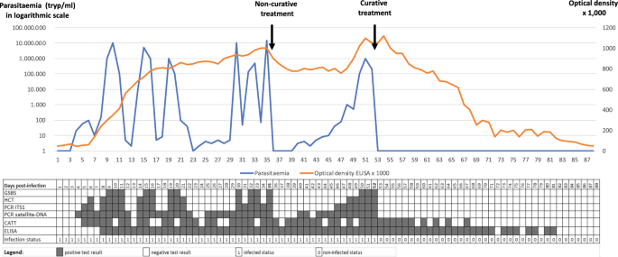
Southern California heat advisory extended as triple-digit temperatures persist in inland areas – Whittier Daily News

A heat advisory for much of Southern California was extended through Tuesday evening, June 28, as a heat wave featuring triple-digit temperatures again dominated many inland valleys Monday.

The advisory, which was previously slated to expire at 8 p.m. on Monday, June 27, was extended an additional 24 hours to caution residents that temperatures well above seasonal averages were expected to persist, the National Weather Service said Monday.

⚠️ Heat Advisory extended through Tuesday evening ⚠️ the heat will hang on through the day on Tuesday across inland areas. Please, use caution and check the back seat of your vehicle when leaving. No child or pet should be left in the car for any amount of time.#CAwx pic.twitter.com/NQbaDz3qDg

— NWS San Diego (@NWSSanDiego) June 27, 2022

In Los Angeles County, valley regions experienced consistent high temperatures between the 90 and 100 degree range, said Rich Thompson, meteorologist with the NWS. Some localities broke the 100-degree mark, including a high of 103 in Van Nuys, Thompson said.

Monday’s heat in the San Fernando Valley was on par with weather there on Sunday during the heat wave. Sunday’s highs included 106 in Woodland Hills and 103 in Van Nuys.

The Inland Empire felt “widespread” highs over the triple-digit barrier, with afternoon readings as high as 108 degrees in Chino and 106 degrees in Riverside and San Bernardino, said Dan Gregoria, meteorologist with the NWS. No daily recorded highs were expected Monday though, he said, due to exceptionally high previous records.

“(Today) doesn’t look like record (high) territory, but it still is hot,” Gregoria said.

Uffda, it is hot out today 🥵 here is a look at our 2:30 PM temperatures. What is everyone doing to stay cool today?#CAwx pic.twitter.com/QNukVj5sJM

— NWS San Diego (@NWSSanDiego) June 27, 2022

Inland Orange County high temperatures ranged from the high 80s to the low 90s, according to Gregoria.

On Tuesday, Inland Empire temperatures are expected to continue hovering around the 100-degree mark, with a slight decrease, Gregoria said. The triple-digit highs are expected to finally recede by Wednesday, June 29, but temperatures in the 90s are still expected inland, he said.

Inland Orange County highs are expected to remain in the 80s Wednesday, Gregoria said.

The decreasing highs are part of a cooling trend that is expected to continue through the Fourth of July holiday weekend, Gregoria said. By Saturday, temperatures are projected to be in the 80s for the Inland Empire and in the 70s for much of Orange County, he said.

Swimmers practice at the William J. Woollett Jr Aquatics Center in Irvine on Monday, June 27, 2022. Orange County and inland areas are under a heat advisory until Tuesday night.(Photo by Leonard Ortiz, Orange County Register/SCNG)

Sophia Gonzales, 2, runs through the splash pad at Heritage Community Park in Irvine, CA, on Monday, June 27, 2022. (Photo by Jeff Gritchen, Orange County Register/SCNG)

While high heat warnings when out over much of Southern California, new surfers honed their skills under cool, foggy conditions at the beach near the Santa Monica Pier Monday, June 27, 2022. High temperatures should begin to subside towards the end of the week. (Photo by David Crane, Los Angeles Daily News/SCNG)

Jackson Staley, 2, grabs a rubber duck toy with instructor Joel Velazquez during swimming lesson on a hot day at Shamel Park on Monday June 27, 2022. (Photo by Milka Soko, Contributing Photographer)

A man hydrates at Cabrillo Beach in San Pedro on Monday, June 27, 2022.
(Photo by Axel Koester, Contributing Photographer)

Naja Rajcic learns to windsurf, taking advantage of windy conditions at Cabrillo Beach in San Pedro on Monday, June 27, 2022.
(Photo by Axel Koester, Contributing Photographer)

Jackson Staley, 2, with instructor Joel Velazquez during a swimming lesson on a hot day at Shamel Park on Monday June 27, 2022. (Photo by Milka Soko, Contributing Photographer)

Michael Elias, 5, gets ready to jump at the pool followed by Magnolia Barkley, 4, during a swimming lesson on a hot day at Shamel Park on Monday June 27, 2022. (Photo by Milka Soko, Contributing Photographer)

Kathy Jiménez, 5, kicks during a swimming lesson on a hot day at Shamel Park on Monday June 27, 2022. (Photo by Milka Soko, Contributing Photographer)

A hover glider takes advantage of windy conditions at Cabrillo Beach in San Pedro on Monday, June 27, 2022.
(Photo by Axel Koester, Contributing Photographer)

Children play in La Pintoresca Park’s newly renovated splash pad in Pasadena on Monday, June 27, 2022 during a heat wave. (Photo by Sarah Reingewirtz, Los Angeles Daily News/SCNG)

Ashanty Tebalan, 6, plays in La Pintoresca Park’s newly renovated splash pad in Pasadena on Monday, June 27, 2022 during a heat wave. (Photo by Sarah Reingewirtz, Los Angeles Daily News/SCNG)

With temperatures soaring past 100 degrees, every piece of shade is precious at the North Hollywood metro station Monday, June 27, 2022. High temperatures should begin to subside towards the end of the week. (Photo by David Crane, Los Angeles Daily News/SCNG)

Ximena Pacheco, 10, plays in La Pintoresca Park’s newly renovated splash pad in Pasadena on Monday, June 27, 2022 during a heat wave. (Photo by Sarah Reingewirtz, Los Angeles Daily News/SCNG)

Children play in La Pintoresca Park’s newly renovated splash pad in Pasadena on Monday, June 27, 2022 during a heat wave. (Photo by Sarah Reingewirtz, Los Angeles Daily News/SCNG)

On Monday, some monsoonal moisture entered the region, producing clouds over the mountains in San Bernardino and Riverside counties with the potential for some thunderstorms, Gregoria said. As of 4 p.m., some of the only precipitation seen had been around the Idyllwild area, Gregoria said.

“If anything (thunderstorm related) would develop, the storms would have the tendency to move into the Inland Empire, like around Hemet,” Gregoria said.

Lightning strikes remained a concern throughout mountain areas for possibly sparking brush fires, but no lightning activity had been reported as of early Monday evening, according to the Angeles and San Bernardino national forests.

At least 15 fires were sparked by lightning strikes in the Angeles National Forest by last Wednesday’s storms, said Dana Dierkes, spokeswoman for the Angles National Forest.

One strike smoldered until Friday, June 24, when it emerged as the 3.5 acre Baldy fire, about two miles west of Mt. Baldy in the remote Sheep Mountain Wilderness, the Angeles National Forest reported. As of Monday, the fire had been 80 percent contained, Dierkes said.

Lisa Cox, spokeswoman for the U.S. Forest Service, warned of “sleeper” fires that can linger after lightning strikes.

“These high temperatures and winds kind of wakes them up,” Cox said.

The threat for thunderstorms was expected to linger with the heat wave as well, with an increased chance for precipitation on Tuesday afternoon, Gregoria said.

Tuesday’s forecasted highs:

After a decade of false starts, Angola finally gets its stock market | Fin24

With about 200 people counting down to Banco BAI’s share debut, Angola’s stock exchange finally got off the ground. 

BAI, the southwest African nation’s biggest lender, had 20 buy orders at 21 650 kwanzas (R760) on the bourse known as Bolsa de Divida e Valores de Angola, or Bodiva, 5% more than the the initial public offering price. But there were no sellers. 

“Today we have reached a new historic milestone,” bourse Chief Executive Officer Walter Pacheco said at the ceremony at the newly built InterContinental hotel. “We come together today to witness the start of a new era for the financial system and the capital markets.”

After more than a decade of delays, the start of trading may help bolster Angolan President Joao Lourenco’s image as a reformer ahead of a general election scheduled for August 24. It could also help spur as many as 20 IPOs in the coming years that aim to attract foreign investment and diversify the nation’s economy away from oil, Pacheco said in an interview late on Wednesday. 

At least two other listings are expected to take place this year – lenders Banco Caixa Geral Angola SA and Banco Millennium Atlantico – before the larger state-owned oil firm Sonangol and Endiama carry out their IPOs, said Pacheco.  

“Hopefully, by 2025, these companies will be in a position to list their shares,” said Pacheco, referring to Sonangol and Endiama. 

There is also a growing interest from closely held companies in a range of sectors to go public, said Pacheco. Angola, Africa’s second-biggest crude producer, has more than 300 companies that have their accounts audited every year, some of which are looking into the benefits of funding their operations through the stock market, he said.

In five to 10 years, Pacheco sees as many as 20 companies trading on the Luanda stock exchange. 

“At first, the stock market will be dominated by financial companies and oil companies, but then we will see a wave of other companies,” said Pacheco. “We won’t be able to compete with Nigeria and South Africa in the next five years, but we are going to be bigger than most stock exchanges on the continent.”

BAI may also offer to sell an additional 10% shares at a later date, bank’s Chief Executive Officer Luis Lelis said at the sidelines of the event.

In times of uncertainty you need journalism you can trust. For 14 free days, you can have access to a world of in-depth analyses, investigative journalism, top opinions and a range of features. Journalism strengthens democracy. Invest in the future today. Thereafter you will be billed R75 per month. You can cancel anytime and if you cancel within 14 days you won’t be billed. 

65 Of The Most Embarrassing Situations People Have Ever Been In, As Shared In An Online Thread – Success Life Lounge

Do you remember the days of playing truth or dare? Sitting in a circle with your best friends at a sleepover, this beloved game was the best way to bond with peers. It was an opportunity to exhibit bravery and vulnerability, while also getting to laugh at your friends as they dove headfirst into silly dares. However, the game did have inherent risks, and in the back of your mind you knew there was always a chance you’d be asked the most dreaded question: what is your most embarrassing moment?

Though we get older, our appetite for embarrassing stories never seems to go away. Last week, Reddit user Konke420xd asked people to share the most embarrassing moments they’ve ever witnessed, and boy, did they deliver. Thankfully for us, this list is a safe space to read other people’s humiliating stories without worrying about our own being exposed, so feel free to laugh as loudly as you want. Enjoy these cringe-worthy stories, and if you aren’t in too much pain from secondhand embarrassment by the end, be sure to check out Bored Panda’s last story featuring mortifying moments right here.

#1

We were doing a math final in junior year of high school. They made a huge deal of saying everyone should use the restroom etc, saying you’d fail if you got out of your seat before your test was done.

About halfway through the exam a girl two seats ahead, and one to the left, starts peeing relentlessly. She didn’t stop taking the exam, look at anyone or try and leave. She released easily 20 oz of fluid. Urine was spilling out of the chair like a faucet for probably 15-20 seconds.

Everyone’s looking at her, the teacher visibly mouths “what the F**K”. No one knows what to do.

This poor girl just finished her exam, probably another 20 minutes’ worth, and left.Image credits: bwchronos

Embarrassment is a feeling we’re all familiar with. Whether you experience it frequently or if you have one particularly painful memory seared into your brain, no one is immune to the feeling. And although many of us hate being embarrassed for obvious reasons, we tend to love hearing other people share their most mortifying moments. Telling friends and family about a painfully embarrassing moment requires vulnerability because, let’s be honest, the reaction is often going to be laughter. But these stories can also be incredibly endearing. Who wants intimidating friends who have never had food stuck in their teeth on a date or waved back to someone who wasn’t actually waving at them? Embarrassing moments are a part of the human experience, and whether we like it or not, they’re just a reminder that nobody can be polished 100% of the time.

#2

I was a sophomore in HS (so around 16) taking the last leg of my county’s sex ed class. It was a co-ed day, so our full gym class of about 30 kids was in the room. Topic was STD’s. The teacher mentioned oral sex a few times and I guess which diseases can be spread through it. One guy who was always pretty quiet and shy raised his hand and said “I just don’t really understand how you can get an STD from talking about sex…”

It took everyone, including the teacher, a few seconds to understand, but some quiet laughter came from a few students. the teacher then of course had to explain as simply as she could that oral sex did not in fact mean talking about sex (I think the stupid bylaws of the program in our county didn’t allow her to fully disclose what it was).

Loading…

Anyway, we thought he was joking but as he heard the laughter from everyone after getting this explained to him, he slowly put his head down and covered his face for the next few minutes. Poor guy. I felt bad, but it was hard not to laugh. At least no one directly gave him s**t for it afterwardImage credits: shlumpy_dumpyyyyy

#3

Alright, so my husband and I were driving around the city and it was pouring outside. Absolutely pouring. We were about to pass the lightrail train tracks (going in both directions) when the crossing gates came down because the lightrail was approaching.

One idiot in a van decided he could make it across before the gates came all the way down. He kept on driving, but he did not make it. Instead, his vehicle was now trapped between the gates.

We could see from our car that this person was PANICKING. His life was flashing before his eyes. In his movie mind, the lightrail was about to crash into the van and drag it for dozens of yards before finally stopping… so he did what anyone would do. He violently pushed the door open and RAN in the pouring rain for his life.

He was halfway down the street before he stopped, turned around, and noticed that the lightrail was patiently waiting for him to move the vehicle. The door was still open. My husband and I just about pissed ourselves laughing.Image credits: JoyceReardon

Now, you may be thinking: I never get embarrassed because I never do anything stupid. And it is true that some people have a higher threshold for embarrassment, but some things are just out of our control. So to anyone who claims they never do anything embarrassing, I raise you some of the following examples from College Times’ list of “Embarrassing Moments We’ve All Experienced”. Ever tried to take a picture of someone else or in a dark room and your camera flash went off? How about this one: accidentally sending a text about someone you know to that person.

Even small encounters that only cause a brief moment of embarrassment count, like going to drink something and spilling it on yourself or tripping while walking down the street. Have you ever walked in on someone using the bathroom, or worse, had someone walk in on you? Maybe your stomach has growled loudly while sitting in a silent room, or you’ve accidentally liked a photo from three years ago while stalking a crush on Instagram. Perhaps you’ve realized halfway through the day that you put on your shirt inside out that morning or accidentally fallen asleep on a stranger’s shoulder on an airplane. Okay, you get the idea. The point is: we’ve all been there.  

#4

I was watching a symphony orchestra concert at the Sydney Opera House one evening. The concert hall foyer has these huge glass windows beneath the sails that overlook the harbourside. The sun hadn’t quite set yet, and every audience member that was exiting the hall could see this incredibly drunk middle aged couple having sex on a bench outside the hall.Image credits: cowbelljazz

#5

A guy making a cringey tap song as a proposal in a public restaurant and getting on one knee only for the girl to go quiet and look around and say “Justin, no! Wtf seriously?” Image credits: SupaDupaDupaDupa

#6

I saw my neighbor get a pizza delivery from two pizza guys (one must have been training) and he must have tried to say “have a great night” and “thanks guys” at the same time and ended up saying “have a great gays!” and the two guys just stopped and looked and my neighbor just shut his door and that neighbor was actually meImage credits: xsc888

Though you may try to avoid it at all costs, embarrassment does not have to be the bane of your existence. Stephanie Vozza wrote a piece for Fast Company explaining “Why Embarrassment Can Be A Good Thing” and even provided some tips on how to handle it. According to Dr. Susan David, a Harvard Medical School psychologist and author of the book Emotional Agility, “Embarrassment is what is called a ‘self-conscious’ emotion; something that we experience in relation to others when we make a mistake or behave in a way that is against social norms or standards.” Though this can be perceived as a negative emotion, it can actually yield benefits. David notes that people who openly feel and express embarrassment are more likely to be trusted and forgiven than people who bottle up their embarrassment.

#7

I used to work in nightclubs. I once witnessed a girl leaning against a wall, casually flirting with a guy and as she laughed she actually s**t herself. She was wearing a white dress and there was no hiding what had happened. The smell actually cleared the whole level of the club. She ran out crying. We had to clean poo off the floor where she had been standing. I often wonder what she is doing now…Image credits: Vaiken_Vox

Election 2022: New vote count shows few questions for local Assembly races – Orange County Register

With only a few exceptions, the vote tallies released late Wednesday for the nine state Assembly seats that touch Orange County now show which primary candidates will advance to the decisive ballot in November.

Here’s a breakdown of the races based on the latest vote counts, along with some context about what might play out in the general election, when turnout is expected to be higher than in the primary and the group of voters slightly more liberal.

In at least two Assembly primaries the final lineup could change over the next few days, when more votes are counted.

68th Assembly District

The most recent tallies suggest it’s all but certain that Anaheim City Councilman Avelino Valencia, a Democrat who works as a district director for retiring Assemblyman Tom Daly, will be one of the two candidates for the seat in November.

It’s less clear who he’ll face.

Republican small business owner Mike Tardif, who’s endorsed by the state GOP, still leads fellow Republican, commercial decorator James Wallace, though not by a decisive number. A fourth candidate, progressive political activist Bulmaro “Boomer” Vicente of Santa Ana, also holds a slim chance of slipping into the run-off field.

Any Republican facing Valencia in November faces long odds. Registration in the district, which includes much of Santa Ana, Anaheim and Orange, favors Democrats by about 30 points.

70th Assembly District

Late vote counts also show a likely primary winner in the Assembly seat centered around Little Saigon. Garden Grove Councilwoman Diedre Nguyen, the only Democrat in a six-candidate field, has held a lead since returns first were announced Tuesday night.

But the latest tallies also suggest at least three of the five other candidates – all Republicans – could finish in the top two. Westminster Mayor Tri Ta is in second, as of late Wednesday, followed by Westminster Councilwoman Kimberly Ho and Fountain Valley Councilman Ted Bui. But the numbers suggest it’s possible for any of those three to finish in second place and move on to the general election.

Two other challengers – Jason Gray, a Westminster city commissioner, and Emily Hibard, a businesswoman from Los Alamitos – appear to be out of contention.

It’s unclear who will be a favorite in November. Registration in the district favors Democrats by four points.

In six other Assembly seats, most primary questions are answered.

59th Assembly District

Three-term Assemblyman Phillip Chen, R-Brea, was the only name on the 59th Assembly ballot Tuesday night, and he has received all of the votes tabulated to date.

But Chen will face an opponent in November. In recent weeks, two residents qualified as write-in candidates – David Naranjo, a 46-year-old Brea resident who owns a real estate appraisal business and is chair of the Libertarian Party of Orange County, and Leon Sit, a 19-year-old engineering student at UCLA who lives in North Tustin and helps run a blog about political data. Whichever of those two gets the most write-in votes – which are expected to be announced late in the vote-counting process – will appear on the November ballot.

The district covers northeast Orange County and Chino Hills in San Bernardino County, and favors Republicans by seven points.

64th Assembly District

The most recent tallies show Republican Raul Ortiz Jr., a pest control manager from La Mirada, and Downey Mayor Blanca Pacheco, a Democrat, are likely to face each other again in November.

But while Ortiz is the leader in the primary, Pacheco probably is the favorite for the general.

The other four candidates – Cudahy Mayor Elizabeth Alcantar, La Habra Councilwoman Rose Espinoza, Norwalk school board member Roberto “Rob” Cancio and Norwalk Vice Mayor Ana Valencia – are all Democrats. And registration in the district, which covers portions of southern Los Angeles County plus La Habra in Orange County, favors Democrats by more than 30 points.

67th Assembly District

Tallies show Democratic Assemblywoman Sharon Quirk-Silva and Republican Soo Yoo, president of the ABC Unified School District’s board, will finish first and second in the primary and face off again in November.

Quirk-Silva is heavily favored to ultimately win a fifth term in the district that covers north-central Orange County along with Cerritos in Los Angeles County and favors Democrats by nearly 18 points.

71st Assembly District

The race in a district that straddles Orange and Riverside counties will feature a rarity in deeply blue California – an all-GOP field in November. The only two candidates in the primary, Temecula Mayor Matt Rahn and Trabuco Canyon activist Kate Sanchez, are Republicans.

Vote tallies show Rahn finishing ahead of Sanchez in the primary, but the numbers are close enough to suggest a competitive race in November. Registration in the district favors the GOP by 10 points.

72nd Assembly District

The latest tallies show what’s been clear since the first votes were announced Tuesday evening: The top two candidates, Democrat Judie Mancuso of Laguna Beach, and Republican Diane Dixon of Newport Beach, are going to finish in a tight race for the top two spots and move on to a rematch in November.

When they do, Dixon, who sits on the Newport Beach City Council, probably is the favorite over Mancuso, who founded a nonprofit that’s helped change laws around animal rights.

Republican Benjamin Yu, a businessman and appointed commissioner in Lake Forest, is in third place in the primary, eating up a share of GOP votes that might go to Dixon in the general election. And registration in the district, which stretches from Seal Beach south to Laguna Beach, plus a narrow carve-out east to Lake Forest, favors Republicans by about six points.

73rd Assembly District

Tallies show two-term Democratic incumbent Cottie Petrie-Norris holding a consistent primary lead over three-term GOP incumbent Steven Choi, but not by a big enough total to define a clear leader heading into November.

But if the primary vote isn’t a hint, party affiliation might be. Registration in the district, which covers Irvine, Costa Mesa, and Tustin, favors Democrats by about 13 points.

74th Assembly District

The outcome of the primary already is clear: GOP Assemblywoman Laurie Davies and San Clemente Mayor Pro Tem Chris Duncan, a Democrat, will advance to the November general election.

After that, the race is a mystery.

Late tallies show Davies leading Duncan, but not by a gap that says anything clear about what will happen in November. The district, which covers parts of south coastal Orange County and a coastal stretch of San Diego County, stretching from Laguna Niguel to Oceanside, is a virtual dead heat in terms of voter registration.

« Previous PageNext Page »